Whereas descriptive statistics are necessary for making sense of the data and exploring it, inferential statistics, especially significance testing is what statistics is all about. The idea of doing statistical tests is related to the discussion on sample: if we have a representative sub-set of a population as our sample, we can make statistical inferences concerning the population on the basis of that sample. These inferences are then generalizable within particular limits, called confidence intervals, that need to be specified.

Confidence intervals

Let us start with a concrete example. In the descriptive statistics section we calculated a mean value for a cropped income variable and got 2782 euros as the overall mean of salaries. The number of observations (n) was 641. If we randomly take one of the cases from the data and check whether that person’s salary is close to the mean, it is likely that it is not exactly the same. There is some distance between the mean and the individual value, either up or down from the mean value. In order to get a picture of all the differences in our sample, we usually calculate the standard deviation, which describes the average distance of data points from the mean. The standard deviation (s) of our salary variable is 913 euros.

Using this information it is possible to calculate the standard error (SE) of the mean, which is a measure of how far the sample means deviate from the true population mean on average from sample to sample. SE is the standard deviation for the theoretical sampling distribution containing all the possible means from all the different samples. According to the central limit theorem (see section Sampling), the sampling distribution is nearly normal and centered at the population mean. The equation for SE is: , i.e. the sample standard deviation divided by the square root of the sample size. This information helps us to define the confidence intervals (CI) for the mean, i.e. the interval within which the true population mean most likely lies.

Let us calculate an example in which we want to be 95% sure about the exact interval within which the true population mean lies. For the upper boundary we add SE multiplied by 1.96 to the sample mean. For the lower boundary we subtract the same value from the sample mean, i.e: . Where does the multiplier “1.96” come from? This value is based on the idea that the sampling distribution is symmetrical, and the value describes the critical limit at both tails of a standardized normal distribution, telling us that there are no more than 2.5% of observations above/below these values. Therefore, the multiplier times SE gives us the limits for mean values that 95% of any sample we could possibly take from the population would yield.

The SE for our sample mean is . Let us calculate the 95% CI for our sample mean: . This allows us to say that in 95 of 100 samples the real population mean value lies between 2711 and 2853 euros, and yet we haven’t done more than one sample! The 95% confidence intervals for the salaries of males and females (these groups have different means, standard deviations, and sample sizes, and hence different standard errors) are depicted in the figure below.

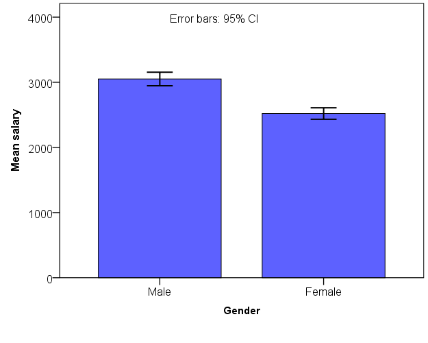
In the figure above the T-bars show the ranges within which the population means for both males and females will fall. The bars show the observed sample means. An important observation is that the error bars are not overlapping, i.e. they do not cover same range of values. This observation makes us more confident in saying that the population means of males and females are different from each other and that the difference is not due to random deviations between different samples.

Testing for a difference between means

In the Theories and models section we briefly touched on the topic of hypothesis testing, when making the distinction between confirmatory and exploratory research. Statistical testing is a method by which hypothesis testing is conducted. Usually we assume the null hypothesis  and the alternative hypothesis . The alternative hypothesis  is what we are interested in. Hypotheses are the research questions that take the form of a “claim”. The null hypothesis is what we test and try to falsify, i.e. to refute by empirical evidence, that is, the data. The statistical test gives us the assurance for saying that the null hypothesis is probably not true, but it also gives us the probability for being wrong (i.e. “risk”) when making such a claim. When we have a reason to suspect the claim of the null hypothesis, then we say that we have found evidence for the alternative hypothesis (if not, however, “proved” it to be true). Most typically,  takes the following form: “there is no difference between A and B” or “A and B are equal”. In turn,  can be expressed in the following way: “A is bigger/smaller than B” or “A is not zero in the population”.

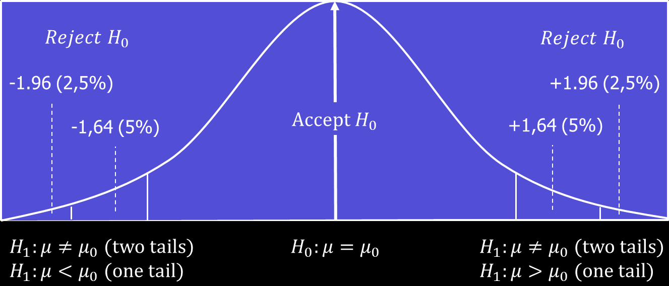
Let us perform a test by which we can be sure that the mean salaries of males and females are different from each other, as the figure above suggested. We begin by setting the null hypothesis : there is no difference between the mean salaries of males and females. The alternative hypothesis  would hence be mean salaries differ from each other. Since we are not testing whether one or the other group has bigger or lower salary, but simply if they differ from each other, the test is called a two-tailed test. The two “tails” refer to the 2.5% tails of the sampling distribution. If we test whether one group’s mean salary is bigger or smaller than the other one’s, we call it a one-tailed test, in which case we would have one 5% tail. The logic of hypothesis testing is illustrated in the figure below, in which there is a sampling distribution with a one and two-tailed tests and regions for rejection and acceptance of the null hypothesis.

To compare two means from independent samples we can use a statistical test called a t-test. The logic is the same as above when we calculated confidence intervals for the sample mean, but this time we use a different formula for calculating how probable it would be to observe a particular difference between the means of the two samples (males and females) given the null hypothesis is true. In our sample the difference happens to be 529.9 euros. The results of the t-test can be seen in the table below.

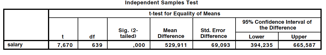
The test starts from the assumption made in  that there is no difference between the salaries, and tests how likely it would be to get 529.9 as the difference given the null hypothesis. It appears that given the sample sizes and standard deviations, it would be nearly impossible to observe such a difference by chance. This is indicated by the t-test value which is 7.670, being way up from the 95% critical value. According to the p-value (“Sig. (2-tailed)” column), less than 0.001% of the all possible samples could generate such a difference. The last columns of the table gives the 95% confidence intervals of the difference, indicating that out of 100 samples 95 will yield a difference between 394.2 and 665.6. Since almost every sample, if properly conducted, would yield such a difference, we have a very good reason to suspect the null hypothesis and hence get support for the alternative hypothesis.

It is good to note that the t-test and the comparison of means is just one type of statistical test. There are many possibilities available, of which the most important are the t-test, F-test and (“chi-sqare”) -test. For example, when doing a contingency table, the test used for examining the statistical significance of the observed differences is the chi-square test. Tests may look different and be calculated differently but the basic idea behind statistical testing is as presented here. The Decision Tree for Statistics is a helpful aid when finding out what statistical test should be used given the data and measurement levels of the variables.