1. Topography of the research area
All the analyses in exercise 4 are focused on Kilpisjärvi and its surrounding area in northern Lapland. The topography analyses were done with digital elevation models (DEMs) of the area. Four different spatial resolutions were used, with pixel sizes ranging from 1 to 10 meters. Both the topography maps (pictures 1-2) are produced with the most precise dataset (DEM1), while the SWI map (picture 4) is, due to long processing times, done with a coarser spatial resolution of 5 meters (DEM5).
1.1. Topographic maps
I visualized two different maps portraying the research area. First, I visualized just the slopes of the area with a simple white to black color gradient (picture 1), and after that tried to form a hillshade map of the area (picture 2). I did not get very representative results with the standard hillshade option, so, instead, I used a custom color gradient (picture 3) on the aspect-analyzed DEM to achieve a do-it-yourself hillshade effect.
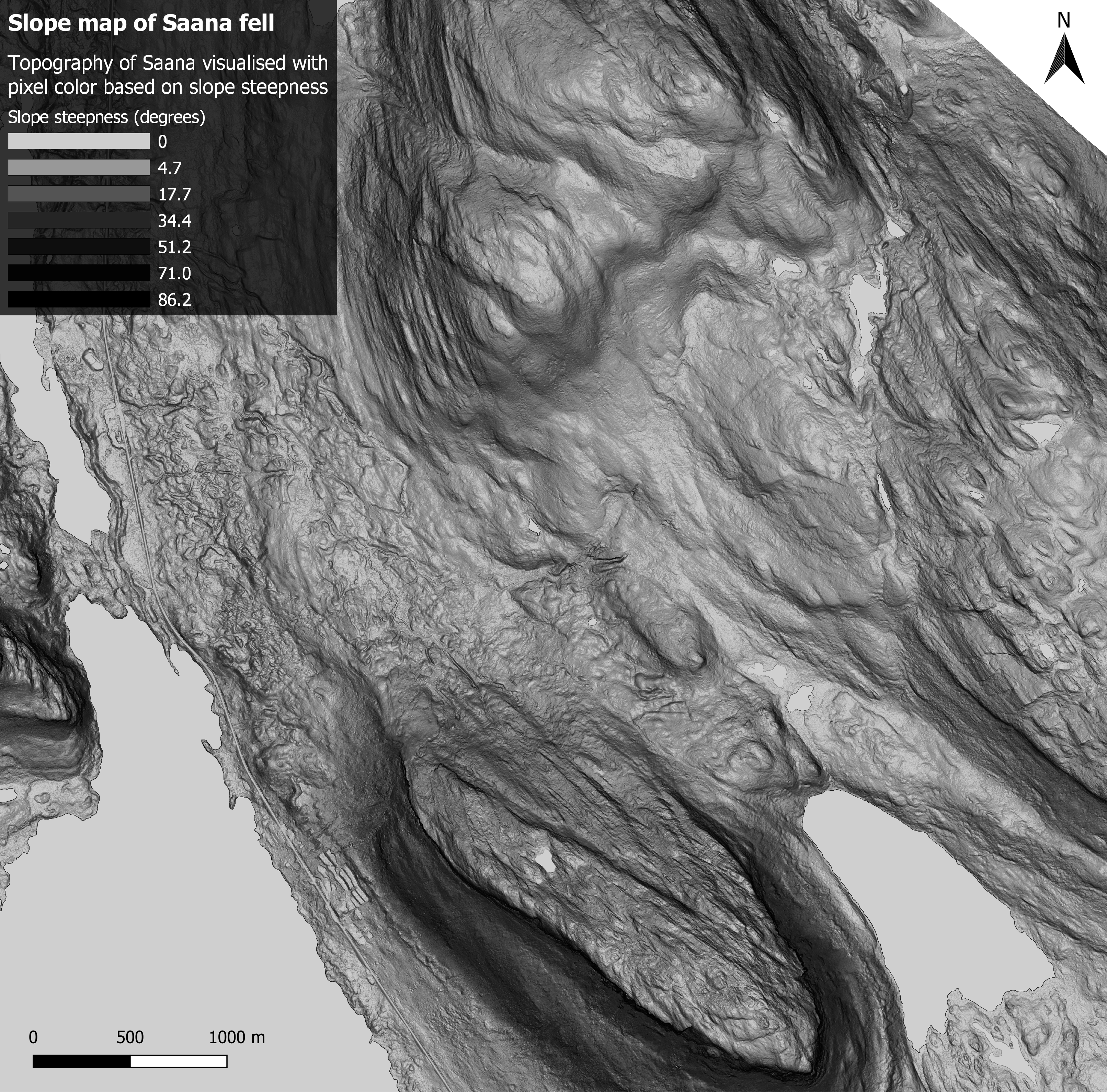 Picture 1. The slopes of Saana. The steeper the slope, the darker the color.
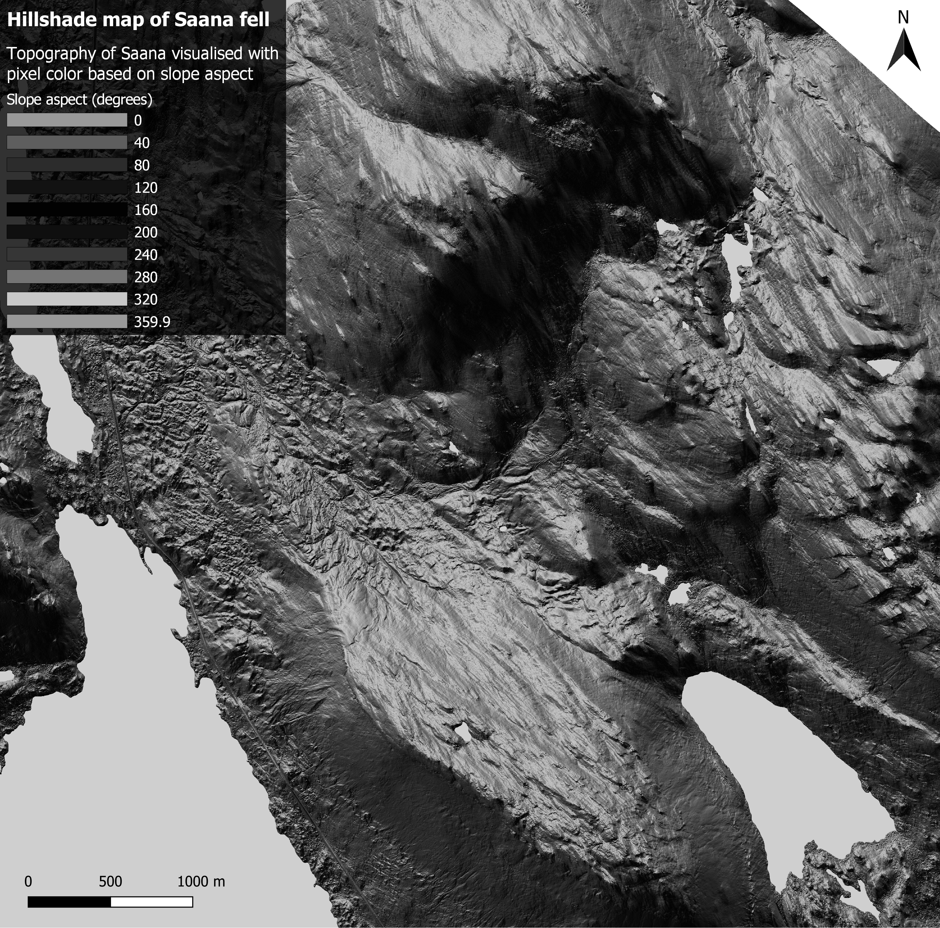
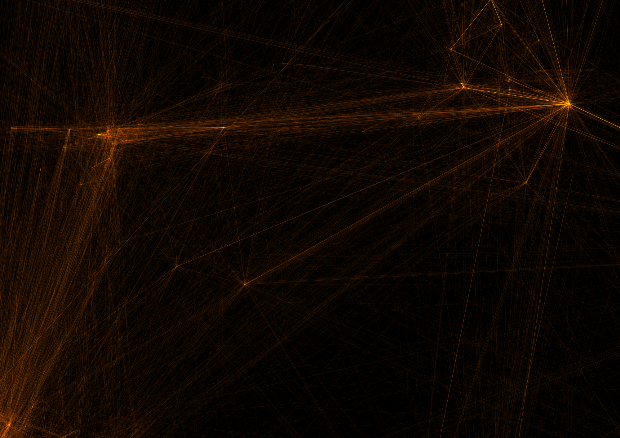
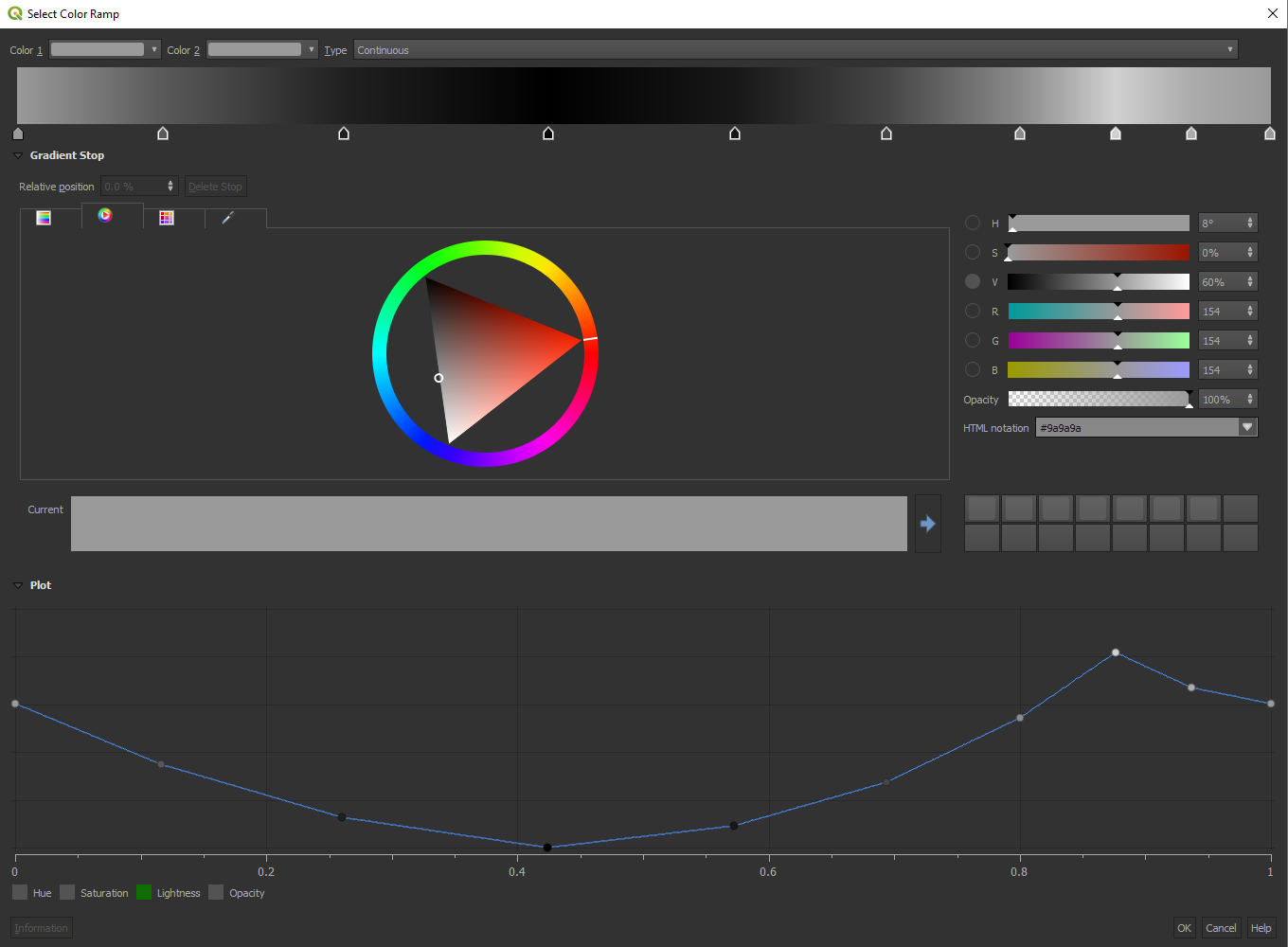 Pictures 2 and 3. The Hillshade map was produced using a custom color gradient. I found out that by moving the light and dark areas on the gradient I could simulate different illumination directions. With this final color gradient variant I tried to simulate the light coming from north-west.
1.2. SWI
Next, the wetness of the soil was calculated using SWI (SAGA Wetness Index).
SWI is a GIS tool that allows the calculation of soil moisture. The operation requires only an elevation model depicting the research area in order to work. The tool is quite reminiscent of the Topographic Wetness Index tool (TWI), but it calculates catchment areas differently: Unlike TWI, SWI does not think of the flow as a very thin film. As a result, it predicts for valley floor pixels that have small vertical distance differences to channels a more realistic, higher soil moisture compared to TWI (SAGA-GIS.org). Below is presented a soil moisture map of the research area, calculated using SWI (picture 4).
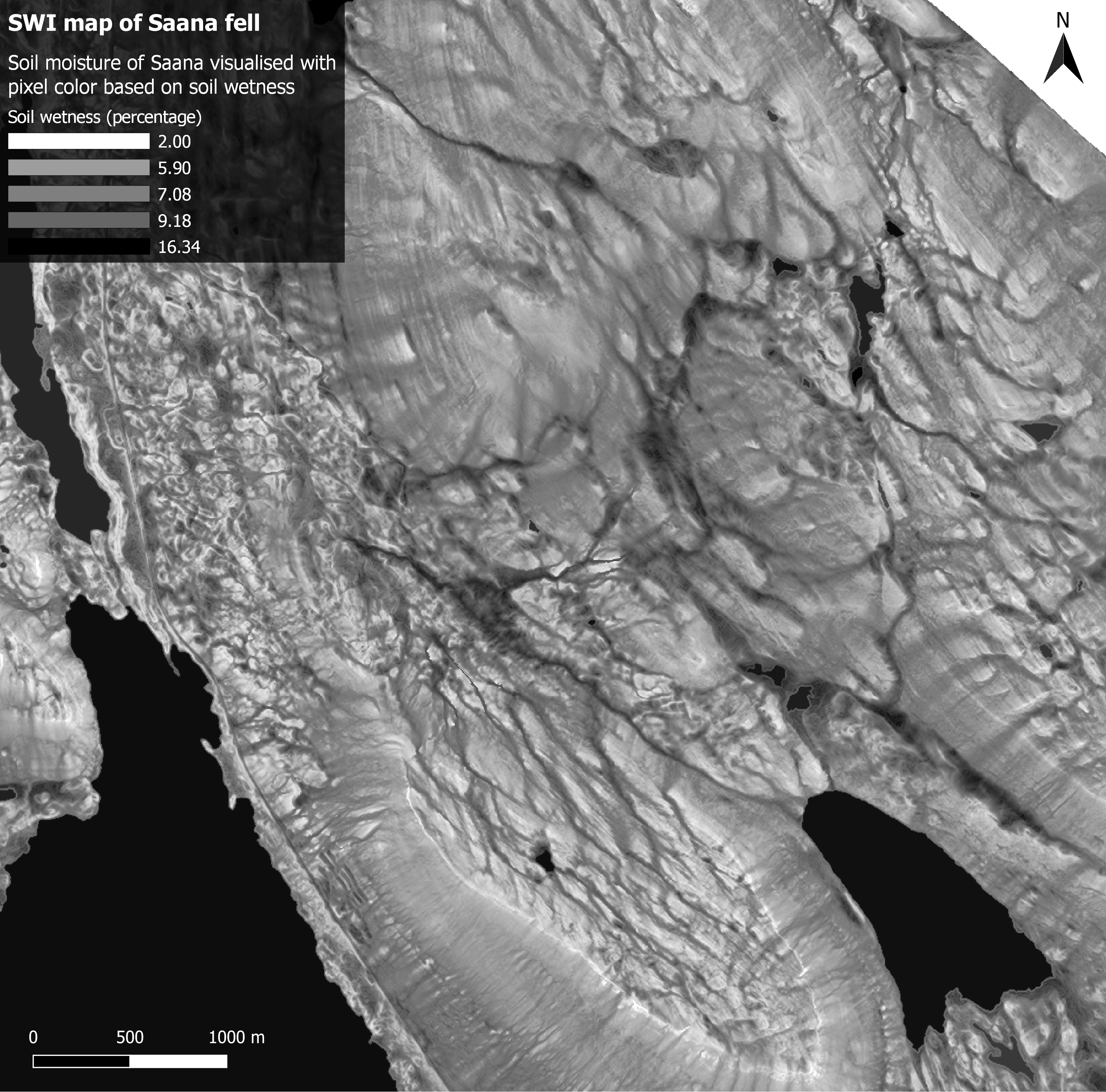
Picture 4. The soil moisture of Saana and its surroundings. Darker pixel color indicates higher moisture percentage.
1.3. Comparison of the SWI and field data
The results of the SWI map were sampled with point sampling plugin and compared to real life samples collected from the same locations. The moisture percentages were also compared to all the topography variables (elevation (DEM1), slope, aspect and general curvature). The correlations between these variables are shown in the below scatter plot matrix (picture 5). It seems that general curvature has the strongest correlation with soil moisture, which is reasonable, as the more curved a surface is, the faster water flows away from that surface point. This is also why the correlation is negative.
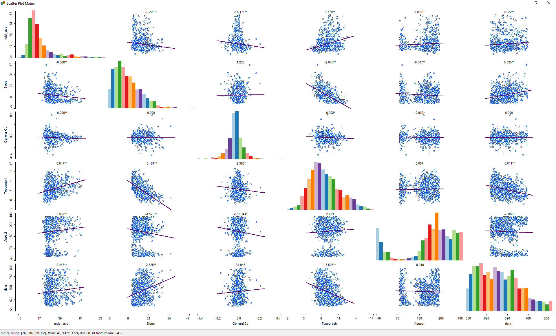
Picture 5. The real-life moisture percentages have a strong negative correlation with general curvature. The next strongest correlation is with the SWI data.
2. Cost surface raster & least cost path
In the second half of the exercise an imaginary rescue operation was planned. An injured fieldworker (called Sakke) is stranded in the Kilpisjärvi research area and the goal is to plan the most efficient rescue route, along which sake can be carried to safety.
The route was constructed with different rasters and ArcGIS’s modelbuilder. The basic work-flow of the route constructing process (picture 6) is to first determine how different terrain types affect carrying a wounded field worker. After this is done, the different layers included in the analysis are changed from vector polygons and polylines to raster format. Once a layer is rasterized, a cost value can be assigned to each pixel based on the type of terrain by reclassifying the layer. Combining the different layers into a single cost surface and then calculating a minimum cost path between Sakke’s location and the location of the rescue points results in three different routes (picture 7).
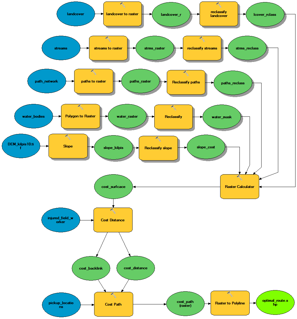
Picture 6. The final model used in constructing the optimal routes. Rock fields, streams and rivers, paths and roads, water bodies and the steepness of slopes are all taken into account in the final paths.
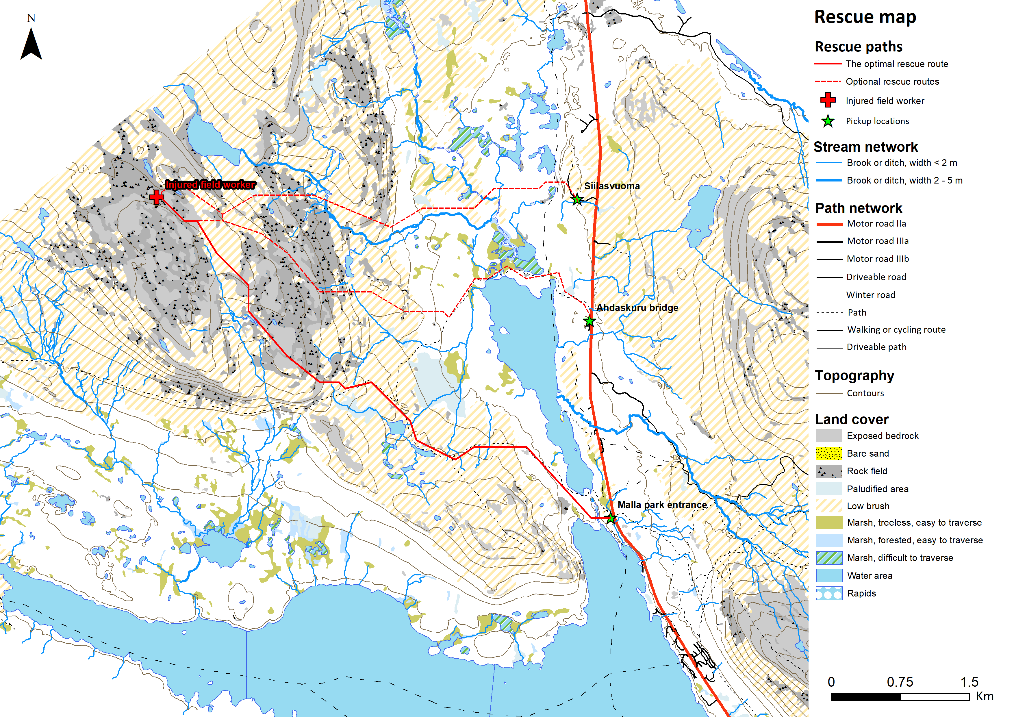
Picture 7. The three rescue routes to save Sakke. The optimal path is drawn as a solid line, while the two other options are dashed lines.
On the finished map, the optimal path ended up leading to the farthest rescue point measuring just by distance (the lengths of the routes are from top to bottom: 5071 m 5729 m and 6708 m). This is the result of the costs I assigned to the pixels: while the path is long, it does not include steep slopes, it goes around the rock fields, and every time it crosses water, it does so along a path. Even the shoes of the commendable rescuers carrying Sakke stay dry!