Metoder inom geoinformatik 2020

The last assignment of the course; Introduction to advanced geoinformatics (spring 2021), was to do a final report about an optional topic and data. I chose to do the final report about the air quality and noise pollution that comes from the traffic in the Helsinki metropolitan area. This is an uttermost important topic as it is one of many reasons for premature deaths and other overall health issues. It is expected that poor air quality and noise pollution will only increase in the future if no solution is achieved.

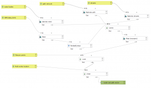
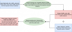
I followed the PPDAC framework as a guideline during the whole process. The framework consists of the problem, the plan, the data, the analysis, and the conclusion. I made this framework prior to the analysis which shows my plan of how to execute the analysis as well as all the inputs (data) and the geoprocessing tools (the analysis) and the desired outputs (conclusion).

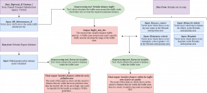
Fig 1. The figure shows my PPDAC framework which lists all the inputs, tools, and outputs.

The problem in the analysis was to locate sensitive features within poor air quality zones as well as within zones with noise pollution exceeding the recommended guidelines of decibel (dB) levels. My plan was to create a buffer zone around busy traffic roads in the Helsinki region with each road’s specific traffic amount deciding the range of the buffer zone. After the buffer zone was created, all the sensitive features that fell within the buffer zone would be extracted. The sensitive features were daycare centres, elementary schools, homes for the elderly, and hospitals.

The road network had information in the attribute table of how much traffic travels daily on each road, and the more daily traffic, the poorer the air quality is next to the road. The sensitive features within the buffer zone are accordingly to HSY (Helsinki Region Environmental Services) too closely located to these roads, due to the high amount of pollution from the traffic that could potentially be harmful to the overall health.  My plan was also to extract all the sensitive features which fell within a zone with a higher than 53 decibel (dB) which is according to WHOs guidelines above the recommended decibel levels.

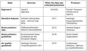
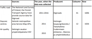
To be able to do this analysis, I used data from many different sources. All my sources have been collected by Finnish municipalities or governmental agencies, so the data is very legitimate. This makes the result of the analysis reliable and accurate. I also followed WHOs noise pollution guidelines “Environmental Noise Guidelines for the European Region” and HSYs air quality guidelines “Air Quality – Minimum and recommended distances for housing and sensitive locations” which are listed in the table below.

Table 1. In the table, there are listed all the sources I used for the assignment, when the data was collected, and who is the producer.

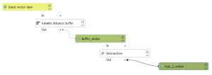
To perform the analysis, I used the graphic builder to build a model that would run the whole process and result in the desired output. I first had to add a new column to the attribute table with the values of the minimum distance from the roads. I had calculated these values using the field calculator. I then used the variable distance buffer tool to create a variable buffer zone with each road’s specific traffic amount deciding the range of the minimum distance buffer zone. When the buffer zone was made around the roads, I used the extract by location tool to see which and the number of sensitive features that fell within the buffer zone. I did also create a layer with the recommended distance from the roads according to HSYs guidelines. I added a new column with the values of the recommended distance to the attribute table and repeated the same analysis.

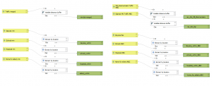
Fig 2. My graphic builder chain at the end of the minimum and recommended distance buffer analysis.

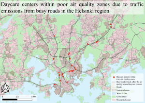
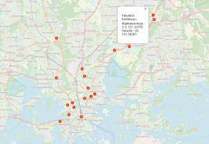
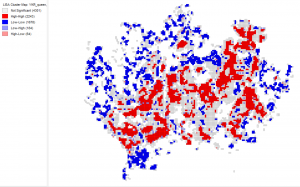
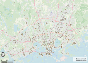
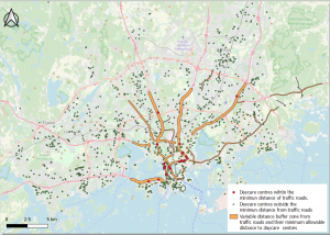
The outcome of the minimum distance analysis showed that only 26 daycare centers, 12 schools, 2 hospitals, and 0 elderly homes of a total of 1483 sensitive features fell within the minimum distance buffer zone. Meaning that these sensitive features are located closer than the allowable distance to a given traffic road because of the poor air quality, according to the HSY report Air Quality – Minimum and recommended distances for housing and sensitive locations. So, the remaining 1443 sensitive features that were in the analysis are located at least the minimum distance from a given road and not affected by traffic pollution and poor air quality to the same extent as those inside the buffer zone.

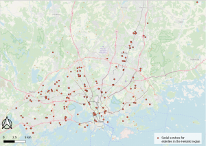
Fig 3. The map shows all the sensitive features within the minimum buffer distance from roads.

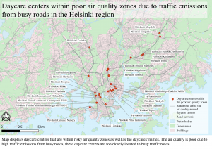
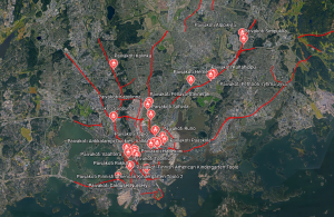
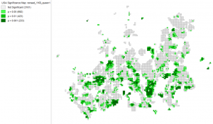
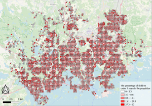
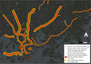
While the outcome of the recommended distance analysis shows that 79 daycare centres, 36 schools, 15 elderly homes, and 3 hospitals fell within the recommended distance buffer zone. Even though these sensitive features do not fall within the minimum distance, they are not in an optimal location if considering the health impacts from the pollution. These sensitive features are below the recommended distance but above the minimum distance, making it a “grey-zone”.

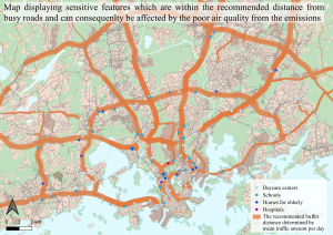
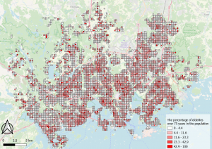
Fig 4. The map shows all the sensitive features within the recommended buffer distance from roads.

When examining figs 3. and 4. a clear pattern can be seen. Most of the sensitive features within the zones are on or within highway ring 3 and with the most focus in the centre of Helsinki. The sensitive features that are the most affected are the daycare centres which have almost as double as many within the sensitive areas as the other sensitive features groups. This is outrageous as daycare centres are for young and undeveloped children that need a safe and healthy environment to grow in.

I did not use the graphic builder to do the noise pollution analysis as it was easier to do it manually with the tools. I started by deleting the fields in the attribute table that had a value below 53 dB so that locations with a decibel over 53 dB would only be visible on the map. Above 53 dB can accordingly to WHOs guideline “Environmental Noise Guidelines for the European Region” be harmful to the health and in this task, I was only interested to see noise polluted areas and which sensitive features fell within. I then used the extract by location tool to extract all those sensitive features that fell within the zone of a higher decibel than 53 dB.

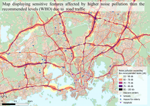
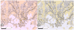
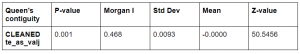
Fig 5. The map shows all areas with noise pollution exceeding 53 dB and the sensitive features within.

Noise pollution due to traffic exceeds recommended levels of 53 dB almost only at greater highways and important traffic roads in the Helsinki metropolitan area. Most of these roads generate an immediate dB level between 75-85 dB right next to the road. The levels of dB rapidly decrease the further away from the road you get. Local factors and variations like buildings, open fields, and specifically built sound barriers also affect the decrease in dB.

There are 184 daycare centres, 43 schools, 20 elderly homes, and 15 hospitals that are within the noise polluted area in the Helsinki metropolitan area out of a total of 1483 sensitive features. This is a legitimate problem as many of the sensitive features which are within the noise polluted areas are also within the poor air quality zone. These sensitive features’ surroundings should immediately be examined and reviewed and solutions to these polluted zones should be achieved at once. Some of these sensitive features could even be potentially moved from the risky areas as it could harm the health of yet undeveloped children and elderly as well as people recovering from an injury. A high amount of pollutions can cause premature deaths and overall health issues as well as social and economic costs (Vieira, J. et al., 2018) and pollution is only expected to increase in the future if no solutions are achieved.

Since pollutions like these are expected to increase in the future, solutions to it are of the uttermost importance. There are different ways to tackle these societal problems, such as nature-based solutions like green-blue infrastructure inspired by nature (Vieira, J. et al., 2018) or strict Air Quality Plans that bring forth a strategy that reduces pollution while is also positive for the economy (Miranda, A. et al.,2015). Local improvements can also be significant in the reduction of local emissions such as speed reduction and street cleaning (Miranda, A. et al.,2015). It is important to define the reasons for pollutions, to be able to solve it. It is not all vehicles that emit large quantities of emissions, the fuel and vehicle type are important variables that need to be considered when reviewing the amount of emissions they emit (Bigazzi, Y. A. & M. Rouleau, 2017). Also, the infrastructure and urban structure and planning are of paramount importance to consider when examining the impacts of pollution. Tightly built high buildings create microclimates that trap pollutions and strengthen them, making the problem even greater.

Due to urbanization and population growth in cities, these societal problem needs to be addressed. These problems could not only lead to an increase in premature death but also to high economic and societal costs in a world that already faces great challenges in the coming decades. Children and the young are the future of this planet and societies so it is very important to protect them from being exposed to pollutants that could potentially harm them. Cities like Helsinki should be front-runners and trendsetters in tackling these societal problems with innovations and new solutions.

References

Vieira, J. et al. (2018) Green spaces are not all the same for the provision of air purification and climate regulation services: The case of urban parks. Environmental Research 160, 306-313.

Bigazzi, Y. A. & M. Rouleau (2017) Can traffic management strategies improve urban air quality? A review of the evidence. Journal of Transport & Health 7, 111-124.

Miranda, A. et al. (2015) Current air quality plans in Europe designed to support air quality management policies.

The sixth week’s theme has been cartographic visualization and interactive maps. It is paramount to visualize maps so that they represent the phenomenon and the result intuitively and correctly. Maps portray different real-world phenomena and can be used for decision-making and even misrepresent information; thus, it is of the uttermost importance that the visualization of the map is suitable for the phenomena. It is as important as any other process in the PPDAC model because ignorant individuals with no previous knowledge of the field can draw assumptions of a phenomenon solely based on how the phenomenon is visualized. So, it is crucial to visualize suitably. Also, when dealing with thematic maps, especially choropleth maps, the classification and the number of classes are very important to consider.

One of the first things to consider when visualizing a map is to answer the question, what is the purpose of this map, and who is the targeted audience? The purpose and the audience define how the map should be visualized. When those questions have been answered, the layout of the map can be defined. The clarity of a map is a key element to consider when visualizing it, it must be clear and understandable for the right audience. What is seen as clarity depends on the audience, if the desired target group is other GIS specialists, then some features on the map can be left undefined as it is expected that the target group has previous knowledge about the feature. While if the audience is newspaper readers, with no expert knowledge about the phenomenon, then the map must have extra clarity for those readers. Another important aspect of map visualization is the visual hierarchy of the different features and elements on the map. Visual hierarchy means that actively choosing which elements to put the most focus on in the visualization, thus which element communicates the main message the most. The balance of the map is also important to take into consideration, for example, how space is used on the map and how features are divided on the map. The balance will influence how well the reader will observe the map and its phenomena. The contrast in the map is also vital to create a visual hierarchy and make certain elements stand out more, though too much contrast can make the map unclear and messy.  The visual unity and harmony of a map is also a key to consider as it affects the reader experience positively and makes the map more inviting and thus more effortlessly to read. There are also some technical aspects to consider, for example, on which platform will the map be published, will it be printed on paper, or stay digital. These aspects will affect, for example, the choice of colours and colour models.

This week’s assignment was to visualize three different maps of the same phenomenon, for three different purposes and thus different target audiences. The data which I visualized was daycare centers that are within risky air quality zones in the Helsinki region. I made one version of the map for a professional publication, one for a newspaper, and one interactive map. The idea of the assignment was to consider how to communicate the main message to the target groups and take into considerations all the elements that make up a good map.

The first map that I made was fictively intended to be published in a professional publication, so the target audience was experts in the field. The main message of the map was to report where these daycare centers are located and the reasons why they are within the poor air quality zone.

Picture 1. Map for an export report publication, it shows daycare centers in risky air quality zones.

Because of the main messages with the map, I decided to put the focus on the daycare centers’ location as well as the busy roads that affect the poor air quality through traffic emissions. I also chose to put rather much focus on the industrial areas on the map as they could potentially increase the amount of emissions in the area. I also focused on visualizing the green areas on the map as vegetation can decrease the amount of harmful emissions in the air. The residential areas are fairly highlighted on the map because those areas also get affected by the emissions. The less significant roads got less attention in the visualization as they don’t directly impact the problem.

I did not define for example, what vegetation the green areas possess since experts are the ones to observe the map, they probably have the knowledge of what kind of environment is typical in southern Finland and the green areas around Helsinki. In addition, the specific vegetation types are not directly relevant to this specific map, even though the vegetation types differ in the amount of emission they can absorb.

I chose earth-like colours to visualize the features on the map as it is pleasing for the eye and is a realistic colour scheme. The daycare centers are visualized with an orange dot inside a red circle to reinforce the message that they are in the risk zone and thus are visualized in typical warning colours.

When making a map for an export report it is first extremely important that all the data and that the analysis methods are correct as the map can be referenced in a report or paper. When visualizing it, it’s important to highlight the essential information of the map as well as cause-and-effect features.

The second map that I visualized was fictively intended to be published in a physical newspaper, so the targeted audience was regular people with no guaranteed knowledge about the phenomenon. This map’s main message was to inform which daycare centers are within the risky air quality zones and inform about the phenomenon as a concept. The reason for wanting to point out which specific daycare centers are within the poor air quality zone is to, for example, inform parents if their children’s daycare center is in a harmful location or not.

Picture 2. Map for a newspaper, it shows daycare centers in risky air quality zones.

Since the main message of the map was to inform which daycare centers are within the risky air quality zones, I decided to put the absolute most focus on the specific daycare centers’ and label their names as well as highlight the busy roads. The other features on the map remain muted since those features weren’t relevant for this targeted audience. In fact, I did combine the residential areas with the industrial areas and refer to them both as buildings for more clarity. The other features basically just created a background map which made the map easier to interpret and read.

When visualizing a map for a newspaper it is immensely important to make a clear map that is easily understood with no features undefined. The visual hierarchy is also very important to consider, as it helps the reader understand the most essential information on the map.

I chose the same earth-like colours as in the previous map for I think the colour scheme is intuitive and nice to look at. Since the map was visualized for a physical newspaper it meant that the map would be printed on paper. This implies consequences for the colours on the map as they use the RGB colour model and printers only print colours in the CMYK colour model. Because of this, I converted all the RGB colour codes to CMYK colour codes and added them to the table below so that the same colours would be achieved when printing the map.

Table 1. The table lists the CMYK colour codes converted from RGB colour codes.

The third map that I made was an interactive map that was fictively meant to be published on the newspaper’s website. This interactive map had the same target audience and message as the previous one but for online readers.

Picture 3. An interactive map for a newspaper website, it shows daycare centers in risky air quality zones.

On the interactive map, I used a pre-made background map and only added the daycare centers’ points to it. Any other features could have easily made the map messy as the purpose of the map is to click on the desired daycare centers and get information on it. In the pop-up window, on the map, I only chose the daycare center’s name and the address information to be visible because the other information in the attribute table was irrelevant for this specific map.

The Daycare centers had the same visualization as before to reinforce the message to the viewer. The background map, OMS Standard, displayed the names of all the districts in the Helsinki region as labels. By displaying the labels, it makes the map more clear and easier to navigate.

When making an interactive map it is important not to add too many features to it as it can easily become very messy when zooming in and out. Another important aspect in the making of interactive maps is that the georeferenced coordinates must be correct, otherwise when zooming in and out the points can shift location which makes the map inaccurate. This is of course very important for any map but especially with interactive ones when the viewer can zoom in very closely.

Picture 4. Screenshot of my interactive daycare centers points in Google Earth.

I also chose to export the daycare centers points and the busy roads as KML files to Google Earth and changed the pin to a daycare center symbol. It was fun to see my produced and visualized data on Google Earth and interactively examine the data with the 3D function.

Picture 5. To the left: Map with a green colourblind lens, To the right: Map with a red colourblind lens

At the end of my visualizations, I exported my maps to the Coblis-website and made a test to see how colourblind individuals would experience my maps. I did the test twice, once with green as the colourblind colour and once with red as the colourblind colour and the results were startling. It was mostly the residential and green areas that were affected by the manipulation which was expected due to their colours on the maps. The green areas changed the most for red colourblinds and could even be misunderstood as fields. If these maps were to be published, I would have changed the colour of the green areas to be suitable for red colourblind individuals as well.

This was by far the most fun assignment that we have done during this course and it felt like I really learned something. I learned both technical aspects as well as how to visualize a map for different purposes. It is truly important to first answer the question what is the purpose of this map and who is the targeted audience? as I mentioned earlier. After those questions have been answered, then the visualization can be defined and proceeded.

This week’s theme has been spatial statistics, focusing on spatial autocorrelation and spatial regression. The idea of the assignment was to observe the spatial autocorrelation’s statistical values and based on those values, draw an assumption of the analysis. I have used QGIS to prepare the data for the analysis, and then I used Geoda for the actual statistical analysis.

Spatial autocorrelation means measuring how one location and its spatial value is related and how similar it is to another location and its spatial value. Positive autocorrelation (+1) is defined as the clustering of the phenomena and their data points. This means that the same values cluster and form groupings. On the other hand, negative autocorrelation (-1) is defined as dispersal of the phenomena and their data points, meaning values are dispersed evenly without any clustering.  Neutral autocorrelation (0) means a random distribution of the phenomena which indicates no correlation between the features.  Spatial autocorrelation is based on Tobler’s first law of geography which states that “everything is related to everything else, but near things are more related than distant things.”. The statistical values the analysis calculates are a z-score and a p-value. These values indicate the statistical significance and whether the null hypothesis can be rejected or not. In spatial autocorrelation, the null hypothesis states that the values are spatially uncorrelated, meaning that the data and the phenomena are randomly distributed. When examining these values, one can determine if the null hypothesis is false or not.

The first part of the assignment was to create a grid and add three columns to the attribute table, named clustered, dispersed, and random. Then I added the values, 5 and 200 to the grid that represented the pattern of the different autocorrelations. I then exported the grid to Geoda where I calculated Morgan’s I. To do a Morgan’s I calculation, the spatial weights have to be added to the layer. I created spatial weights with both rook’s and queen’s first contiguity. After this step, I was able to perform the Global Morgan’s I calculation which generated the z-value as well as the p-value of the autocorrelations.

Table 1. The table shows the p-value, Morgan’s I, standard deviation, mean, and z-value of the autocorrelations when using Rook’s contiguity.

When using Rook’s contiguity, both clustered and dispersed columns had a p-value under 0.05 which means that they are statistically significant and that the null hypothesis can be rejected. While the random column had a non-significant p-value, meaning that the null hypothesis cannot be rejected. This was expected because random autocorrelation implies that there is not a correlation between the features. The z-values on the other hand varied a lot. Z-value is the standard deviation of a normal distribution. A very high or low z-value indicates that it is not likely that the feature of the pattern is distributed randomly, which is what the null hypothesis says.  In summary, a high or low z-value in combination with a significant p-value, states that the null hypothesis can be rejected, and the distribution of the features is not random. By observing the values in table 1., one can draw the conclusion that clustered and dispersed columns are not randomly distributed, which is true.

Table 2. The table shows the p-value, Morgan’s I, standard deviation, mean, and z-value of the autocorrelations when using Queens’s contiguity.

The statistical values changed when using Queen’s contiguity. The only column which was significant was the clustered one that had a p-value under 0.05. The z-values did also vary quite much but only the clustered z-value did indicate a rejected null hypothesis.

It is interesting how the values changed when changing contiguity, I am not completely sure why they changed but I guess it has something to do with the number of neighbors and grid cells that they calculated.

Picture 1. Three spatial correlograms. To the left: Random spatial correlogram.  At the middle: Clustered spatial correlogram. To the right: Dispersed spatial correlogram

From the correlograms, it can be observed the pattern of the feature’s distributions. For example, the clustered spatial correlogram, clearly shows two clusters, one with a higher value and the other with a lower value.

In the second assignment, the idea was to use this previous knowledge to do a statistical analysis of a real-world phenomenon. I did the analysis on the occupancy rate of households in the Helsinki region. First, I weighted the spatial weights with the queen’s first contiguity. I then calculated the global Moran’s I. The p-value of the data was below 0.05, meaning it is statistically significant as well as a high z-score which supports it. This means that the occupancy rate of households is not randomly distributed, instead they are clustered.

Table 3. The table shows the p-value, Morgan’s I, standard deviation, mean, and z-value of the autocorrelations when using Queens’s contiguity.

After calculating the global Moran’s I, I calculated the local Moran’s I which resulted in one significance map and one cluster map. From these maps, the phenomenon can be observed more easily, as it is more intuitive. On the significance map below, the four categories tell how significant the result is in the area in the analysis. So, the dark green areas on the map, have a high significance, meaning the results of these areas are close to the actuality. While the bright green areas on the map have a p-value just on the significance borderline, meaning the results of these areas are less trustworthy. The grey areas are not significant, meaning these areas are not to be trusted in the clustered map (picture 3).

 

Picture 2. Significance map of the occupancy rate of households in the Helsinki region. It was easier to interpret the map without any background map so I chose not to add one to my report.

The significance map is meant to be observed with the cluster map seen below. The clustered map shows the areas where there is a high and low occupancy rate relative to the number of inhabitants in a household. The red areas on the map, show locations where there is a high occupancy rate while the blue areas show where there is a low occupancy rate. The bright blue colour show outliers, which are locations where there is a low occupancy rate relative to the surrounding areas which have a high value and vice versa with the bright red category. The significance map tells which of these clustered areas are very significant and thus more trustworthy as well as which areas are less significant and trustworthy.

When observing the cluster map, there are certain areas where the result seems a bit inaccurate. For example, Suvisaaristo is a detached house area but according to the cluster map, there is a low occupancy rate which is inaccurate. While Westendi and Kauniainen have, according to the map, high occupancy rates which is accurate.

Picture 3. Cluster map of the occupancy rate of households in the Helsinki region. It was easier to interpret the map without any background map so I chose not to add one to my report.

Since there were some inaccuracies in the previous Moran’s I calculation, I had to trim certain values from the data in QGIS. I trimmed all the No data values as well as the cells that hadn’t any neighbors and then I calculate the Moran’s I again.

Table 4. The table shows the p-value, Morgan’s I, standard deviation, mean, and z-value of the autocorrelations when using Queens’s contiguity.

The p-value for the trimmed dataset was also significant with a p-value of 0.001 and a high z-score. So the null hypothesis could once again be rejected. When examining the new significance map which the latter analysis gave, it can be observed that the area that the map portrays is much smaller than in the previous analysis. The most significant areas are the Kallio district, Kauniainen municipality, and Westendi in Espoo as well as some other locations.

Picture 4. Significance map of the occupancy rate of households in the Helsinki region. It was easier to interpret the map without any background map so I chose not to add one to my report.

The cluster map has also changed a lot when using the trimmed dataset, it is more accurate than the previous cluster map. Now distinct neighborhoods can truly be observed and a clear pattern can be seen.

Picture 5. Cluster map of the occupancy rate of households in the Helsinki region. It was easier to interpret the map without any background map so I chose not to add one to my report.

The municipality, Kauniainen, is a former villa community with a higher than average square meter per capita, thus large houses are scattered around within the municipality borders. According to the cluster map, there is a high occupancy rate that fits in with the urban space of Kauniainen. The same goes for Westendi, which is also an area with large houses scattered around in a wider space.  The district of Kallio has a low occupancy rate, meaning there are fewer square meters per capita and inhabitants live densely. This cluster result fits in with the urban space of Kallio as it has many one-room apartments because it has once been an important district for the working-class with cheap small apartments.

The map below visualizes the occupancy rate in the Helsinki region but is made in QGIS. The red areas have a lower occupancy rate while the green areas have a higher.

Picture 6. The map that shows the occupancy rate in the Helsinki region

The third part of the assignment was to do yet another spatial autocorrelation analysis with another real-world problem. In this part, I used data columns of children under the age of 7 and elderly over the age of 75 to see if these age-groups cluster and if so, where. The idea was to do the analysis in percentage, and in that way acknowledge the proportional amount of the age group in the population.

In the earlier stages of the assignment, I had done several spatial autocorrelation analyses, so the concept was at this stage familiar. I started by writing my analysis plan that consisted of first; data trimming and calculation of new variables in the attribute table, then the global Moran’s I followed by the local Moran’s I calculations. I then analyzed my results and visualized maps. After all these stages, I could draw a conclusion.

I started by trimming the datasets with cells that had no No-data and cells that had no neighbors in QGIS instead of doing this at a later phase. I then calculated the proportion of children in the population as well as the elderly. I then added the values to new fields in the attribute table. I exported the managed data to Geoda where I did the actual analysis. I started by weighing the spatial weights of the variables with both queen’s and rook’s first contiguity. I then calculated the global Moran’s I and the results were expected. The p-value for both variables was under 0.05 when using both queen’s and rook’s contiguity and the z-score was also relatively high. This means that there is not a random distribution of children and elderly in the Helsinki region, they are either clustered or dispersed.

Table 5. The table shows the p-value, Morgan’s I, and z-value of the autocorrelations when using Rook’s contiguity.

Table 6. The table shows the p-value, Morgan’s I, and z-value of the autocorrelations when using Queens’s contiguity.

I then calculated the local Morgan’s I with only the weighted queen’s contiguity for both variables. This analysis resulted in a significance map and a cluster map.

Picture 7. Significance map of the children’s proportion relative to the population in the Helsinki region.

Picture 8. Significance map of the elderlies proportion relative to the population in the Helsinki region.

These significance maps are a little unclear in my opinion because many pixels are undefined and only a very small proportion is significant, especially in the significance map portraying children’s proportion.

The cluster maps below, show the clustering of the age groups and where these clusters are located. Red areas show where there is a high amount of clustering of the given age group while blue areas show where there is a low amount of clustering. While the bright blue or bright red shows outliers which implicates locations, which have a different value than their surrounding areas.

Picture 9. Cluster map of the children’s proportion relative to the population in the Helsinki region.

When the cluster maps are examined, different patterns can be observed in the clusterings. Children’s proportion is lower inside the Helsinki municipality, especially in the Kallio district. In the previous task, the results indicated that there is an overall low occupancy rate in Kallio which seems to fit in with this result. There is a higher proportion of children in the Kauniainen, Espoo, and Vantaa municipality, especially in the west.

I chose to make a map of daycare centers of the data we used in the first week to see if there is a correlation between the clusters and daycare centers. There are many daycare centers in the center of Helsinki, but the children’s proportion is low in the cluster map there due to the otherwise high population.  In Kauniainen and in Espoo there are many daycare centers that seem to correlate with the clusters as well as in Myyrmäki in Vantaa. Almost all daycare centers are located close to road networks. The same factor can be observed from the cluster map, where children’s proportion is higher closer to road networks.

Picture 10. The map shows daycare centres in the Helsinki region

I did also make a map of the proportional distribution of children under the age of 7 in QGIS. This map also shows that there is a higher proportion of children in the population outside the Helsinki city center. That which this map adds to the analysis is that there is a very low percentage of children in the more rural places, towards north, northwest, and east. When observing the map of daycare centers, one can see that they decrease in that direction and that may be the reason for the low proportion of children in those areas.

Picture 11. The map shows the percentage of children in the Helsinki region.

Picture 12. Cluster map of the elderlies proportion relative to the population in the Helsinki region.

The cluster map of elderlies’ proportion in the population shows clear clustering and areas where there is low clustering of elderly. According to the cluster map, elderlies are clustered for instance in Westendi, Kauniainen, Myyrmäki, Kumpula and Käpylä. What all these locations have in common is that they are near services but not in the CBD and that they are near green urban spaces. More rural places north and northwest has a lower clustering of elderlies. This pattern could also be seen with the proportional distribution of children. The reason for this is that there are fewer services in rural areas which affects the attractiveness negatively for families with children and the elderly who often are dependent on services. Even though clusterings are found both in children’s and elderlies distribution, elderlies cluster even more according to the results of the analysis.

Picture 13. The Map shows all kinds of social services for the elderly.

I did also make a map that shows every social service for elderlies in the Helsinki region. When examining the cluster map, correlations can be seen with the distribution of social services for elderlies and their clustering. There is a clear correlation between the social services and the clustering’s which seems logical and expected.

I did a map of the phenomenon in QGIS which also supports the analysis made from the cluster map and the map that shows the distribution of social services for the elderly.

Picture 14. The map shows the percentage of elderly over 75 years in the Helsinki region.

 

This week’s topic has been raster analysis, focusing on digital elevation modeling and how to do a least-cost path analysis. A least-cost path analysis calculates the shortest, most optimal, and cheapest route from a destination to a source when no network exists. The analysis weights the different inputs and calculates which of those inputs costs more and which of them costs less. This means that some obstacles in the terrain are harder to cross than others, meaning it impacts the cost of the path and thus changes the route. In the analyses, I have used SAGA and GRASS software’s which are integrated with QGIS.

The first part of the assignment was to calculate the slope and aspect degree as well as the curvature of a digital elevation model in the Kilpisjärvi region. This was made with the SAGA terrain analysis geo algorithms. I also calculated the topographic wetness index with the SAGA wetness index (SWI) algorithm. Saga Wetness Index is an index that calculates the soil moisture in a given location. The index is based on the “Soil regionalization by means of terrain analysis and process parameterization” by the EUROPEAN SOIL BUREAU. The SWI algorithm is based on terrain analysis, parameterization, soil regionalization, and then process modeling which is described further in the article. To perform an SWI, a digital elevation model needs to be as elevation input. Also, the type of area and slope must be specified as well as suction. This algorithm results in a topographic wetness index.

The exploratory data analysis shows that there is a positive significant correlation between topographic wetness index and soil moisture. This correlation means that if one of the variables increases or decreases, so does the other variable as well. Therefore, topography affects the soil moisture, for example, if there is a depression in a landscape, there is most likely moist soil in the depression whereas at a hilltop the soil is probably less moist.

Picture 1. Diagram showing correlations between the variables.

The first least-cost path analysis that I made was with the plugin, least-cost path. It resulted in three paths that don’t take the terrain into consideration. These paths aren’t realistic and therefore I continued the analysis with different methods.

Picture 2. The map shows the least-cost paths when the analysis was made with the plugin

In the second analysis, I used the graphic builder to build a model that took the terrain and different obstacles into consideration when calculating the least cost path. First, I made an analysis where I only used water bodies and slope as inputs, which generated the green route on the map below. Then I ran the model again, this time with water bodies, slope, and also the path network as inputs. This model did also take the path network into consideration when calculating the least cost path which is the dark red route on the map below. Lastly, I made a third analysis where I yet added streams to the model. This resulted in a model that also took streams’ size into consideration, it is the blue route on the map below.

Picture 3. The map shows three different least-cost paths which have different inputs. The inputs used in the calculation of the least-cost paths are listed beneath the symbol.

I calculated the length of all the least cost routes which are listed in the legend on the map. The route which also took the streams into consideration was the shortest route while the route that took the path network into consideration was the longest.

To create a least-cost path analysis, first, a cost surface has to be made. I made the cost surface with the r.series function, which is a raster grid that possesses the cost value of the inputs in each cell. Then a cost distance has to be made, which I made with the r.cost function. Cost distance is a continuous layer with the cumulative cost determining the movement between cells. Lastly, the least-cost path analysis can be made with the r.drain function which I used. Instead of the r.drain function, the r.walk function can also be used to achieve the same results.

This part of the analysis took many hours to complete because the graphic modeler ran for hours before completing the task. At the end of the analysis, the model was quite complex, with many rasterized inputs and functions.

Picture 4. What my model looked like at the end of my analysis.

I did also make a least-cost path with the knight’s move activated in the cost distance section. The knight’s move means that the output will be more accurate but that the process might be slower. Knight’s move doubles the cost distance which means that it covers more grids, meaning that the cost distance with the knight’s move is more comprehensive.

In this least-cost path analysis with the knight’s move activated, I only had water bodies and slope as inputs so the model ran quite fast because of few inputs. The output of this analysis can be compared with the least cost path with the same inputs that I mentioned earlier in picture 3. The map below shows both the least-cost paths with and without the knight’s move and their difference. There is a clear difference between the paths even though they are quite similar. The white path shows a more accurate route, it is 5568 meters long which makes it the shortest route between the injured field worker and the pick-up locations.

Picture 5. The map shows both the least cost path with and without the knight’s move.

Sources:

BÖHNER J., KÖTHE R., CONRAD O., GROSS J., RINGELER A. and SELIGE T. (2002) Soil regionalisation by means of terrain analysis and process parameterisation. Pages, 213-221. EUROPEAN SOIL BUREAU. RESEARCH REPORT NO. 7. https://www.researchgate.net/publication/284700427_Soil_regionalisation_by_means_of_terrain_analysis_and_process_parameterisation

https://helpmanual.io/man1/r.cost-grass/

This week’s topic has been analyses, focusing on network analysis in GIS. We have read and discussed different topics in network analysis such as usage, terminology, algorithms, and functions. The most known and used algorithm in network analysis is called Dijkstra’s algorithm which is based on the mathematical graph theory.

In this week’s assignment, the task was to get familiar with the network analysis methods and concepts and use different tools and functions to solve routing problems as well as to calculate distances to nearby objects. To complete this exercise, I have used different queries, tools, and functions as well as observed statistics and combined different databases and layers.

The first part of the assignment was to create the shortest bicycle route from Porthania to Kumpula campus using the Dijkstra algorithm. I calculated both the distance, as well as the time of travel from Porthania to Kumpula campus. This analysis was made with queries which are listed below in table 1.

Table 1. The table lists the queries I used when creating the shortest route from Porthania to Kumpula campus. The algorithm is based on Dijkstra’s algorithm.

I did the same analysis twice, in the second analysis, I used a different function. The second function I used, shortest path, is a QGIS providing network analysis function. To perform the shortest path analysis, the start and end vertex need to be chosen from the map, I chose Porthania as the start vertex and the end vertex as Kumpula. I also added a few variables, such as the digitization direction of the roads which affected the outcome of the analysis.

The routes that the two analyses gave were quite identical except for one minor difference. The start of the route differed. The first analysis route started from the Yliopistonkatu and went along the Fabianinkatu to Kajsaniemikatu. The second analysis route also started from the Yliopistonkatu but went along the Vuorikatu instead of Fabianinkatu to Kajsaniemikatu. This was the only noticeable difference between the two analyses.

Picture 1. The map showig the shortest route from Porthania to Kumpula using Dijkstra algortihm

Picture 2.The map showing the shortest route from Porthania to Kumpula using the“shortest path”tool

The differences between the analyses are minor which also can be seen in the statistics below in the table. According to the statistics of the analyses, the distance varies slightly as well as the time of travel. The first analysis with Dijkstra’s algorithm has a vaguely longer distance between the start and end vertex than the second analysis. This is probably because of the difference in the start of the route, where the route through Vuorikatu is longer. The time of travel varies by about 5 seconds between the routes so the difference is very insignificant.

Table 2. The table shows the statistical differences between distance and time in the two different network analyses.

A part of the assignment was to create the shortest bicycle route from Pasila train station to Viikki, Kumpula, Porthania, and Aalto campuses. I calculated the time of travel and distances from the station to the campuses with the Dijkstra algorithm. I used the same queries as before (table 1.), besides I changed the start and end vertices for every campus. The Pasila train station is where all the lines meet in the centre of the map and the campuses are at the end of the lines.

Picture 3. The map shows the shortest path from Pasila train station to the four different campuses calculated with the Dijkstra algorithm

In the table below, I have listed the distances from Pasila train station to the campuses as well as the time of travel. In the assignment, the students arrived at Pasila station at 12 pm so their expected time of arrival is also added to the table. The time of travel was given in minutes but the numbers were in a decimal numerical system. To make it more clear, I converted the decimal numbers into minutes and seconds and then rounded them off to whole minutes.

Table 3. The table shows the differences in route distance and time as well as the time of arrival. The minutes have been rounded to whole minutes for more clarity.

Another task in the assignment was to create hub distances portraying the shortest linear routes from city bike stations to public transport stations. I used the distance to the nearest hub tool to calculate the shortest linear distance. The linear distance doesn’t tell much of the real transport route distance because of the line’s linearity but it gives the relative distances which can be useful when e.g. determining the distance between countries or facilities. The linear distance can also be useful for flight routes and planning infrastructure facilities.

Picture 4. The map shows the hub distance from city bike stations to public transport stations.

Because the linear distance doesn’t tell much of the transport route distance, the second part of the task was to create the distances of routes along the road. These distances were measurably longer than the linear distances.  To be able to perform this analysis, I first made an OD Matrix of all the possible connections between vertices, and then I performed an execute SQL query which calculated the shortest route distances when taking the transport network into consideration. The query I used, is listed in the table below.

Table 4. In the table is listed the query I used to calculate the distances of routes along the road.

Picture 5. The map shows the shortest linear and route distances from city bike stations to public transport stations

Some city bike stations had a shorter route distance to another public transport station than what the linear distance had suggested. Different obstacles, like infrastructure or construction sites and the environment and so forth, can block the linear distance, thus making the actual route longer. This is fairly normal when it comes to the difference between linear and route distances which needs to be taken into account when calculating distances.

The route distances are useful in navigation and when determining the absolute travel distance with a car, bicycle, or public transport.

I also observed the statistical differences between the two analyses. The values vary a bit, which is expected due to linear distances are often shorter while the route distances are often longer.

Table 5. The table displays the mean, min, and max statistical differences between the linear and route distance.

The last part of the assignment was to create a layer that displayed the city bike stations’ service area with a 500-meter radius and the number of residents within the area. I used the service area tool to create the polygon and afterward, I used the convex hull tool to extract all the YKR centroids within the service area’s polygon. The result of this could be seen in the attribute table, which showed the number of residents inside the service area. Within the service area, there were 457 952 residents.

Picture 6. The map shows the service area with a 500-meter radius from the city bike stations.

The results of this extensive analysis were quite realistic. The bicycle routes from Pasila train station to the campuses differed a little bit with Google maps suggested routes and expected travel times. A reason for this may be that Google maps only suggested roads, while my analysis did take walkways into consideration. For example, according to my analysis, the shortest route from Pasila to Kumpula was through Kumpulantaival garden, which is a walkway where motor vehicles aren’t allowed. Google maps don’t suggest this route at all, maybe because the service only suggests roads or roads that have a specific bicycle lane. Data quality is also an important element in network analyses, as incomplete data can severely change and affect the outcome of the network analysis.

Bicycle routes can differ from cars route quite a lot because of the possibility to cycle through places where motor vehicles aren’t allowed. This is important to take into consideration when determining the shortest route and the difference between a motor vehicle and a bicycle route.

 

During the second week of the course, Introduction to advanced geoinformatics, we have read and discussed big data, data-driven geography and started using the Structured Query Language, SQL. Since big data and data overall have been on the tapestry this week, we have especially focused on the quality of the data. Data quality is vital for every analysis and task, imprecise and inaccurate data can change and affect the analysis negatively which makes data exploration very important.

This week’s exercise was to explore data, using SQL queries and assess data quality. The data I worked with, was location-based Flickr data containing information about users, photos, and activity on Flickr posts in the Helsinki region.

Table 1. A table with basic statistical information about the Flickr database. In the table, there are listed all the values of the statistics and the queries used to collect the values.

The first part of the assignment was to collect basic statistical values from the Flickr database. To do this, I used different SQL queries in the PostGIS application in QGIS. In the table above (table 1.), I have listed all the queries I used and the statistical results that the queries gave.

After I had collected the statistical values, I exported the Flickr database to a QGIS project. The database showed locations of Flickr posts on the map in QGIS. I visualized a point pattern map, to display the locations of Flickr posts in the Helsinki region. The locations of the posts are scattered around in the Helsinki region, with a concentration within the highway ring III.

Picture 1. The map shows all the separate locations of Flickr posts in the Helsinki region.

I also visualized a heatmap of the Flickr database that shows the concentration of Flickr posts’ location in the Helsinki region. According to the point pattern map and the heatmap, the vast majority of the 126 010 posts are located in the centre of Helsinki.

The popular tourist hubs, Helsinki Cathedral, market square Helsinki and Suomenlinna are hotspot locations for Flickr posts, according to the heatmap. Also, Pasila, with Messukeskus, Linnanmäki and Hartwall arena as well as Töölö, with Helsinki Ice Hall and The Olympic Stadium are popular places for Flickr posts. Tapiola and Matinkylä are places with a rather high amount of Flickr posts while most of Espoo and Eastern Helsinki are places that have a smaller amount of posts. Nuuksio National Park and the Helsinki-Vantaa airport are distinct places outside the highway ring III, which are locations for Flickr posts although in a small amount.

Picture 2. The map shows both hotspots, where there are the highest concentrations of Flickr posts as well as locations, with a less concentration of posts.

After I had visualized a point pattern map and a heatmap of the database, I continued the task by combining the Flickr database with a grid polygon with the size of 500x500m. This was a challenging process, as it was hard to figure out the exact query to combine those two. After trying for about an hour, I got help from the instructor who helped me solve the query. In the table below, the query is listed which I used when aggregating the data.

Table 2. The table shows the query I used to aggregate the Flickr database and the grid polygon 500x500m.

When I finally got the database and the grid combined, I visualized the result as a thematic map. Because of the wide differences between the concentrations of posts’ geographical locations, the classifications of the thematic map were a bit tricky. As I earlier mentioned, most of the posts’ locations were in the centre of Helsinki while surrounding areas had a much smaller concentration of posts. This made the classification of the thematic map rough because there were places with few posts and places with many thousands of posts.

Picture 3. A thematic map of the aggregated data, that shows the amount of Flickr posts per grid 500x500m

The last part of the task was to choose a specific location in Helsinki and check the accuracy of the location in the posts. I chose Korkeasaari Zoo as my location and made the analysis twice, once with the Flickr database and once with the Instagram database. I used a string of queries to extract all the locations that mentioned the word “Korkeasaari” in the posts’ text description, and those posts’ latitude and longitude as well as their geometry. This formed a new layer with points representing the location of each post that somehow was connected to the word “korkeasaari”. The queries I used to extract the specific locations are listed below in the table.

Table 3. A table that shows the queries I used, to extract all the location points that had the word “korkeasaari” in the text description.

Just because a specific location or place is mentioned in a post on a social platform, it does not necessarily mean that the post is from that exact location. The reasons for this can be many. When analyzing results from large databases with the help of queries, that aren’t specific enough, it’s important to acknowledge the fact that the results can possess places that aren’t relevant for the analysis. Different geographical places can have the same names, which can make analyses based on names or words vague.

It was interesting to see how the results varied significantly between Flickr and Instagram databases. The Instagram database had a lot more points that were connected to the statement word ‘%Korkeasaari%’than Flickr database had. The map below (picture 4.) shows Flickr posts locations and distance layers. Almost all points are on the actual Korkeasaari Zoo island while one point is on another island, also called Korkeasaari.

Picture 4. A map that shows the actual location of Korkeasaari zoo and Flickr posts locations where “korkeasaari” is mentioned as well as distance layers between the actual place and the locations of the posts.

There are much more Instagram posts mentioning “korkeasaari”, and the points are also scattered around in a much bigger area than Flickrs’ posts. Instagrams’ post locations are concentrated around the centre of Helsinki but many posts go as far as Espoo and even Järvenpää. I am unsure of the reason for this. Is it because the GPS of the posts is weak or are there many places around Uusimaa named “Korkeasaari”? This is the key reason why analyses based on words can be vague.

Picture 5. A map that shows the actual location of Korkeasaari zoo and Instagram posts locations where “korkeasaari” is mentioned as well as distance layers between the actual place and the locations of the posts.

Table 4. A table that shows the statistical difference of the location accuracy between Flickr and Instagram database. The min and max distance is in meters.

In the table above (table 4.) I have listed the statistical differences between the accuracy of the locations in the databases. When performing comparisons like these, it’s important to examine the statistical values to determine the difference between the accuracy.  When inspecting the statistics, a Flickr’s post’s max distance from Korkeasaari zoo is 9169 meters while an Instagram post’s max distance from the zoo is 33 346 meters. When examining the maps (pictures 4 and 5), one can see that the furthest point from Korkeasaari Zoo in the Flickr database is in the Helsinki archipelago, which is about 9170 meters from the zoo. While the furthest point from the zoo in the Instagram database is in Järvenpää, which is about 33km from Korkeasaari zoo. The other values are quite the same between the two databases although there are considerably more points in the Instagram database. In this analysis, measurable qualities can be seen, for example, the accuracy of the location as well as the precision, while non-measurable qualities don’t appear as much in the analysis. This comparison has really opened my eyes what regards data quality. It is truly important to investigate and explore the data prior to analysis, to see if the data is suitable or not.

I have certainly learned a lot from this exercise, even though it took a long while and was difficult and frustrating at times, but most importantly, it felt meaningful doing the assignment.

This week’s theme, Geospatial analysis as a process, focused on how to use the graphic builder (alt. Model builder) as an automating tool in geospatial analysis. Graphic builder is a tool that helps design, perform, and automate geoprocessing tasks. A Graphic builder consists of an input, algorithm/process, and output. The input is the file or data one wants to use for the analysis, the algorithm is the geoprocessing tool that performs the analysis, and the output is the result of the analysis. Graphic builder is very helpful when dealing with large datasets with a long analysis process with many different inputs, geoprocessing tools, and outputs.

In this week’s assignment, the task was to create a buffer zone around busy traffic roads in the Helsinki region. With each road’s specific traffic amount deciding the range of the buffer zone and then extract those daycare centres that fell within the buffer zone. Each road had information in the attribute table of how much traffic travels daily on the road, and the more daily traffic, the poorer the air quality is next to the road. The daycare centres within the buffer zone are accordingly to HSY (Helsinki Region Environmental Services) too closely located to these roads, due to the high amount of pollution from the traffic.

During the whole process, I used the PPDAC framework. The framework consists of the problem or reason for the analysis, the plan, the data, the analysis, and the conclusion. I made this framework before the analysis which shows my plan of how to execute the analysis. In the framework, I listed all the inputs (data) and the geoprocessing tools (the analysis) which I used, and the desired outputs (conclusion).

Picture 1. The pictures show my PPDAC framework which lists all the inputs, tools, and outputs for the exercise

To be able to do this analysis, I used data from many different sources. All my sources have been collected by Finnish municipalities or governmental agencies, so the data is very legitimate. This makes the result of the analysis reliable.

Table 1. In the table, there are listed all the sources I used for the assignment, when the data was collected and who is the producer as well as the number of columns and rows in the attribute table that each dataset had.

I used the variable distance buffer tool to create a variable buffer zone with each road’s specific traffic amount deciding the range of the buffer zone. When the buffer zone was made around the roads, I used the intersection tool to see which daycare centres fell within the buffer zone. At the beginning of the task, I suffered from some technical issues, the variable distance buffer tool couldn’t find my chosen input vector layer. I asked the instructor for help and she helped me to locate the problem, then the graphic builder ran successfully, and an output emerged. Afterward, the analysis went on without a problem. Because of the frustration at the beginning of the assignment with the technical issues, I’ll grade this exercise a 3 on the difficulty scale. The idea of the assignment and what geoprocessing tools to use weren’t hard to figure out, but the technical aspects of the program and the graphic builder were somewhat more challenging. Below is my graphical builder chain when the analysis was completed.

Picture 2. This is how my graphic builder chain looked like at the end of the analysis.

The outcome of the analysis showed that only 21 out of 1026 daycare centres fell within the buffer zone. Meaning that these daycare centres are located closer than the allowable distance to a given traffic road because of the poor air quality, according to the HSY rapport Air Quality – Minimum and recommended distances for housing and sensitive locations. So, the remaining 1005 daycare centres were located at least the minimum distance from a given road and not affected by traffic pollution and poor air quality to the same extent as those inside the buffer zone.

Almost all of the 21 daycare centres within the buffer zones are located in the centre of Helsinki, next to important and busy highways and less busy traffic hubs. Within the centre of Helsinki itself, most of the daycare units affected by poor air quality, due to traffic emissions are located within the districts of Kallio, Sörkkä, and Töölö. Mechelininkatu, Helsinginkatu, Länsiväylä, Mannerheimintie, and Mäkelänkatu are the most important roads that affect the daycare unit’s air quality the most.

Picture 2. A map of the Helsinki region shows daycare units within the buffer zone as well as daycare units that are outside the buffer zone and the buffer zone itself.

In the optional assignment, the task was to create a new field in the attribute table with the values of the recommended distances from traffic roads. I used the field calculator to calculate the recommended distance. This resulted in a new field, with the recommended distance. Afterward, I made a variable distance buffer analysis in the graphic builder with the new field

as the distance field. I also used the intersection tool to extract daycare units, which were within the minimum distance as well as within the recommended distance, so-called the “grey zone”.

The red squares in the map below portray the daycare centres which are within the risk zone, and the green squares portray those daycare centres which are between the minimum distance and the recommended distance, which I call the “grey zone”. The smaller white dots show daycare centres that are well outside the recommended distance, and thus not affected by the pollution from the traffic emissions. The red buffer zones show the minimum distance, whilst the yellow buffer zones show the recommended distance from traffic roads.

Picture 3. The map shows daycare centres within, between and beyond the minimum, and recommended distances from traffic roads as well as the minimum and recommended buffer zones.

During these exercises, I learned how to use the graphic builder in Quantum GIS as well as add a new field to the attribute table. I haven’t used QGIS for about a year now, so the exercises did also refresh my memory and skills in QGIS.

As of now, the following posts will be weekly exercises from the course “Introduction to advanced geoinformatics”.

Så är de sista uppgifterna avklarade för denna kurs. Jag tycker att kursen har varit givande, meningsfull och jag har definitivt lärt mig en hel del om GIS programmet, ArcGis Pro. Kursen har behandlat många viktiga och användbara teman och analyser samt byggt en stark grund för framtida fördjupade geoinformatik kunskaper.

Denna vecka har vi fortsatt med temat interpolering och fördjupat oss i olika tillvägagångssätt i hur man väljer interpolerings metoden och verktyget för en speciell analys. Ofta används interpolering då man skall mäta olika fenomen i naturen men det är orealistiskt att mäta exakt varje punkt i terrängen. Oftast har man data från enskilda specifika observationspunkter och dessa punkter används som grunden till interpoleringen. Med hjälp av olika matematiska funktioner kan man göra välgrundade gissningar och förutspå värdet på ett område som inte har blivit mätt. Dessutom kan man räkna osäkerheten och sannolikheten för att gissningen är felaktig. Detta skapar ett pålitligt interpolerings lager som visualiserar kvantitativa variabler av t.ex ett fenomen i naturen. I och med att det finns flera interpoleringsmetoder är det ytterst viktigt att välja rätt metod då man gör en interpolering, annars kan resultatet bli felaktigt och visa skevhet. En metod för att veta vilken interpolerings metod som anpassar sig bäst för analysen kan räknas ut med att titta på variablerna; medelvärde, standardavvikelse, standardfel och kvadratiskt medelvärde samt av att iaktta cross validation grafen och verktyget.

I första uppgiften Interpolate temperatures using the Geostatistical Wizard skulle man skapa en kontinuerlig temperaturkarta över Afrika och Mellan Östern från punkt data. Jag använde både Inverse Distance Weighting och Kriging interpolerings metoderna för att skapa olika lager. Jag skapade två stycken IDW lager och två stycken Kriging lager. Sedan jämförde jag dessa fyra lager för att avgöra vilket var det lämpligaste lagret som motsvarade verkligheten mest. För att avgöra detta iakttog jag bland annat variablerna; medelvärde, standardavvikelse, standardfel och kvadratiskt medelvärde samt iakttog cross validation grafen.

På kartan nedan ser man ett tydligt naturgeografiskt mönster på temperatur skillnaderna. Öken områden så som Sahara  och Arabiska öknen befinner sig vid högtrycksbältet som har ett nästan konstant högtryck över sig med väldigt lite årlig nederbörd. Detta skapar en hög genomsnittlig medeltemperatur i området vilket synns på kartan. Sahel området söder om Sahara är en halvtorr gränszon som har något svalare klimat och mera nederbörd. Denna region ser man tydligt på kartan. Regnskogsområden vid ekvatorn har ett tropsikt klimat med väldigt mycket nederbörd och då också ett lite svalare klimat på grund av de konstanta lågtrycksbälte som befinner sig ovanför ekvatorn. Sydafrika som är beläget mer sydligt har ett subtropiskt klimat med svalare  temperatur. Längst kusten går den kalla bengualaströmmen vilket ger upphov till torrt och svalt klimat.

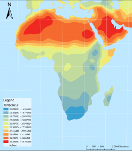Karta 1. En interpolerad karta över temperaturskillnader i Afrika och Mellan östern. ArcGis PRO.

Jag skapade också ett kartlager som visar standard felet av resultatet. Då lade jag de observerade punkterna på kartlagret för att ytterligare visa korrelationen mellan standardfel och områden som inte har blivit mätta. Ju mörkare färg, desto högre standardfel. Man ser ett tydligt geografiskt mönster på kartan. Vid mer svåråtkomliga områden finns det betydligt färre obervationspunkter, t.ex Sahara öknen och Kongo-Kinshasa regnskogsområdet. Dessutom finns det nästan inga obervationspunkter i både Somalien och Jemen vilka är två krigszoner, den samhälliga situationen i dessa länder påverkar säkert möjligheten för att få pålitlig data.

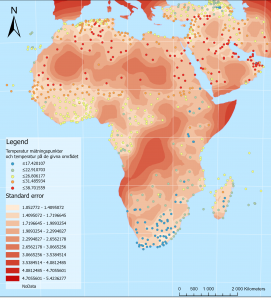Karta 2. En karta över standardfelen av temperatur gissningarna i den föregående kartan (karta 1.). ArcGis Pro.

Denna modell visar arbetsskeden i uppgiften. Den blåa rutan föreställer den givna datan och de röda ovalerna föreställer verktygen jag använde. De gråa ovalerna är specifika kommandon jag gjort inom verktygen som har haft en stor effekt på resultatet. Till sist visar de gula rutorna skapade lager medan den gröna rutan, Kriging Modified föreställer de lager vars resultat förställde verkligheten mest och hade bland annat minsta standardfelet. Alltså Kriging Modified interpoleringslagret valde jag att visualisera och ha som referenskarta för temperaturskillnader i Afrika och Mellan östern.

Bild 1. En modell på arbetskeden i uppgift 1. 

I den andra uppgiften Analyze Urban Heat Using Kriging skulle man skapa ett interpolerat kartlagret över stadsdelar i staden Madison, Wisconsin. Kartlagret skulle visualisera effekten av urban värmeö och visualisera temperaturskillnaden mellan centrumområdet i Madison och mer avlägsna områden runt staden. Sedan skulle man räkna ut vilka stadsdelar som har mer än 100 000 invånare som är över 65 år och bor i stadsdelar där medeltemperaturen är högre än ca. 27 grader celcius. Höga temperaturer under en längre tid kan vara en hälsorisk för åldringar, enligt Svenska Yle (den finskavärmeböljan har börjat kräva dödsoffer – hettan kan fortsätta i fyra veckor framåt 25.07.18) ökar långvariga värmeperioder dödligheten hos åldringar med 20% därför är det ytterst viktigt att prioritera åldringar under en värmebölja samt planera eventuella åtgärder. För att myndigheterna skall kunna förutspå och planera åtgärder för eventuella värmeböljor måste man först kartlägga dessa akuta områden. Då är interpolering ett utmärkt verktyg för att räkna ut och visualisera dessa områden samt var åldringar bor och i hurdan kvantitet inom riskzonen.

För att slutföra denna uppgift använde jag olika interpolerings metoder för att skapa olika lager. Dessa lager jämförde jag sedan för att avgöra vilket kartlager motsvarar verkligheten bäst (jag använde samma metoder som i första uppgiften för att avgöra vilket kartlager hade lägsta standardfelet).  Sedan använde jag diverse olika verktyg (se modellen nedan) för att skapa det slutgiltiga resultatet.

Modellen nedan visar arbetsskeden i uppgiften. De blåa rutorna föreställer data jag använde i uppgiften och de röda ovalerna föreställer verktygen jag använde. De gråa ovalerna är specifika kommandon jag gjort inom verktygen som har haft en stor effekt på resultatet. Till sist visar de gula rutorna skapade lager medan den gröna rutan längst ner är resultatet över temperaturskillnader mellan stadsdelar samt utmärker stadsdelar där det bor fler än 100 000 åldringar över 65 år.

Bild 2. En modell på arbetskeden i uppgift 2. 

Stadsdelar vars gränser är avgränsade med blå färg är stadsdelar som har en medeltemperatur över ca. 27 grader och 65 årigar vars invånarantal överstiger 100 000, detta kan man se från kartan nedan. Dessa är stadsdelar som myndigheterna bör övervaka under värmeböljor. Man ser tydligt att centrala business disriktet har högst temperatur vilket kan förklaras av urban värmeö fenomenet. Städer som är tättbebyggt med mycke betong, mörk asvalt och lite grönska har låg albedo effekt vilket innebär att de absorberar mera energi än reflekterar. Då stiger temperaturen på dessa byggnader och infrastrukturen vilket skapar en värmeö.

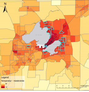Karta 3. En interpolerad karta över temperaturskillnader i stadsdelar i Madison, Wisconsin samt stadsdelar som har fler än 100 000 invånare som är äldre än 65 år. 

 

Källor:

Granskog, S. 24.07.2018. Den finskavärmeböljan har börjat kräva dödsoffer – hettan kan fortsätta i fyra veckor framåt. Svenska Yle.https://svenska.yle.fi/artikel/2018/07/24/den-finska-varmeboljan-har-borjat-krava-dodsoffer-hettan-kan-fortsatta-i-fyra

Brander, N. Hiekka, S. Paarlahti, A. Ruth, C. Ruth, O. Zenit, Den blåa planeten. 2016) 

Denna veckas tema bestod främst av att lära sig använda 2D och 3D interpolation verktyg samt förstå vad korsvalidering är och hur algoritmen skall läsas. Jag tyckte inte värst mycket om denna veckas uppgifter, de kändes tråkiga och väldigt teoretiska.

I den första uppgiften ”Model Water Quality Using Interpolation” skulle man med hjälp av interpolation verktyget göra två interpolations kartor över mängden upplöst syre i Chesapeak Bay estauriet i östra USA år 2014 och 2015. Låg syrehalt i hav under en längre tid kan skapa syrefritt botten vilket innebär att det inte finns något syre på havsbottnet. Arter kan inte leva i dessa omständigheter vilket leder till artutdöd. En viktig anledning till syrefria havsbotten är övergödning; stora mängder näringsämnen hamnar i havet och ökar algproduktionen. Då algerna dör sjunker de till bottnet där nedbrytningsprocessen förbrukar syre. Orsaken till övergödning är antropogen verksamhet, bland annat utsläpp av avloppsvatten, gödsel från jordbruk eller avverkning av skog. För att minimera artutdöd till följd av syrefria botten är det ytterst viktigt att följa med syrehalten i vattendrag. Med att mäta syrehalten i vattendrag kan man med hjälp av geoinformatik skapa diverse kartor och grafer som visar tillståndet av vattendraget. Interpolation är till exempel ett sådant verktyg som lämpar sig utmärkt för att visualisera och analysera syrehalten i vattendrag.

Uppgiften bestod av att först göra ett linjediagram och ett histogram för att iaktta syrehalten i estauriet under ett kalender år. Det visade sig att under sommarmånaderna var syrehalten lägst. I och med den låga syrehalten fokuserade uppgiften på sommarmånaderna för att granska vattentillståndet för den perioden.

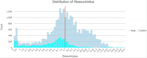Diagram 1. Ett histogram över syremättnaden i Chesapeake Bay. ArcGis PRO.

För att skapa interpolations kartlagret från 2014 använde jag mig av Geostatistical Wizard för att slutföra analysen med interpolations with barriers verktyget. Detta skapade ett nytt interpolations kartlager där mängden syre i estauriet visualiserades med hjälp av en färgskala. Jag använde en annan metod för att genomföra interpolations analysen på vattentillståndet från år 2015. Via geoprocessing aktiverade jag verktyget kernel interpolation with barriers där jag slutförde analysen. Resultatet blev också en interpolations karta där syrehalten i vattendraget visualiserades med en färgskala. I uppgiften bekantade jag mig även med hur viktigt det är att välja rätt storleks omkrets runt alla observerade punkter för att uppnå en interpolations karta vars skala på värden löper jämnt.

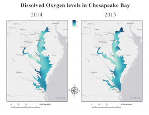Bild 1. Två kartor som visar syremättnaden i Chesapeake Bay sommaren 2014 och sommaren 2015.  ArcGis Pro.

Syrehalten I Chesapeake Bay hade inte en enorm skillnad mellan sommaren 2014 och sommaren 2015. Med hjälp av korsvalidering kunde man estimera prediktionsfelet i analysen.

Bild 2. Arbetsskeden och verktyg  i analysen ”Model Water Quality Using Interpolation”.

I den andra uppgiften skulle man göra en 3D geostatistisk interpolation på syrehalten i Monterey Bay, Kalifornien. Jag använde geoprocessings verktyget Empirical Bayesian Kriging 3D för att skapa de interpolerade kartlagren över syrehalten i havet. I denna uppgift gjorde man många små ändringar och det fanns många steg för att uppnå resultatet. Resultatet blev en animation av 3D kartlagren över syrehalten i havet.

När man iakttar resultaten visar det att syrehalten är högst närmast havsytan medan syrehalten sjunker rejält enda till 800 meters djup vartefter syrehalten ökar igen. Jag vet inte vad orsaken till detta är men det är absolut ett intressant resultat.

Andra delen av uppgiften bestod av att visualisera resultaten i ett voxel lager. För att skapa ett voxel lager använde jag GA Layer 3D To NetCDF verktyget. Det var relativt lätt att skapa lagret men uppgiften handlade mycket om hur man redigerar lagret och förändrar det visuellt. Till sist skulle man skapa isosurfaces av syremättnaden i havet.

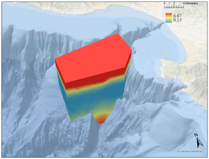Bild 3. Ett voxel lager som visualiserar syremättnaden i Monterey Bay, Kalifornien. ArcGis Pro. 

 

Källor:

Sveriges meteorologiska och hydrologiska institut, SMHI. Syreförhållandet i havet. 14.01.2014. https://www.smhi.se/kunskapsbanken/oceanografi/syreforhallanden-i-havet-1.5155

Sveriges meteorologiska och hydrologiska institut, SMHI. Källor till övergödning. 17.08.2009. https://www.smhi.se/kunskapsbanken/oceanografi/kallor-till-overgodning-1.6011