I will post relevant links and info relating to my poster at the Star@Lyon conference. This page will be updated during the conference if e.g. questions are asked.

Email: emma.mannfors (at) helsinki.fi

About me:

PhD student at the University of Helsinki (supervisor: Mika Juvela)

Click here to download my poster (650 kB)

This poster is based on two papers:

• Juvela, M., and Mannfors, E., 2023, A&A, 673, A145​
  • ADS link
• Mannfors, E., Juvela, M.,  Liu, T., and Pelkonen, V.-M., submitted.

Contents

1. Observations
2. Data reduction
3. Important concepts
4. Other images in the poster
5. References

Observations

We have observed OMC-3 (Orion Molecular Cloud 3) with three instruments:

Instrument​	Wavelength​	Resolution​
​	(µm)​	(”)​
Herschel SPIRE​	250, 350, 500​	20​
APEX ArTéMiS​	350​	~10
Spitzer​	8​	2​

Table 1: The instruments used in this paper. Also see Fig. 1

Fig. 1: OMC-3 column density maps with Herschel (left), ArTéMiS (center), and Spitzer (right). θ is the beamsize of the instrument. The filament path in each field is marked by the line. Segments A-D were also extracted for the HR and AR data. 

How did we get the ArTémis (AR) map?

​Observations (350 um) with ArTéMiS were combined by feathering with the 350 um SPIRE Herschel observations, using the program uvcombine.

Using feathering, we have data with higher-resolution, smaller features and large-scale structure visible with Herschel.

Data analysis

Calculating N(H2) for our data

HR: We used the modified blackbody (MBB; see below) function to estimate temperature, optical depth, and column density using Herschel SPIRE 250-500 um data.

To achieve a resolution of 20″, we used the method described in Palmeirim et al., (2013; Appendix A).

AR: We used the feathered 350 um intensity map (resolution: ~10″) and Herschel temperature maps (resolution: 20″) to estimate column densities.

Modified blackbody (MBB)

(For more info on MBB fitting, see e.g. Mannfors et al., 2021. Direct ADS link on my research-> papers page)

The MBB describes IR emission and is described by the formula:

(B_{nu}(T) / B_{nu, 0}(T) ) * (nu / nu0)**beta

Where B_{nu}(T)  is the Planck function at frequency nu, and beta is the opacity spectral index.

Beta = 1.8 is fairly accurate in dense clouds.

Plummer profile:

(Arzoumanian et al. 2011; André et al. 2014).

We have used a modified version of this where both sides of the profile are fitted separately, with  N₀  kept constant.

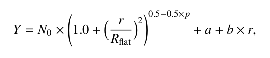
Where N₀ = the maximum intensity / column density of the filament

r = the distance from the center of the filament

R_flat = the width of the filament

p = the slope of the filament

a + br = linear background

 

Other important concepts

0.1 pc width

See e.g. Arzoumanian et al., 2011,  André et al., 2014

Images in the poster

Observations

Fig. 2: Width (FWHM) of the filament segments.  A-D correspond to the segments in Fig. 1 (right). The full field filament is shown in Fig. 1 (left,center). ​

Simulations

 

Fig. 3: Derived widths for a simulated filament, as a function of column density and assuming an ISRF like Mathis et al., (1983; X=1, yellow squares), 10 times stronger (X=10, red circles), and 100 times stronger (purple triangles).  ​

 

Fig. 4: Simulations on the effect of distance to a simulated filament. (left): The components: a random sky background (purple solid lines), a large Gaussian component to simulate hierarchial structure (orange dashed lines), and a Plummer-like filament (purple dotted lines). The resulting profile (at a simulated distance of 500 pc) Is shown with solid orange lines, and the Plummer fit with dashed black lines. (right): Violin plots of filament distance vs. Filament width. ​

References:

Mannfors, E., Juvela, M.,  Liu, T., and Pelkonen, V.-M., subm.

Juvela, M., and Mannfors, E., 2023, A&A, 673, A145

André, P., Di Francesco, J., Ward-Thompson, D., et al. 2014, in Protostars and Planets VI, ed. H. Beuther, R. S. Klessen, C. P. Dullemond, & T. Henning, 27

Arzoumanian, D., André, P., Didelon, P., et al. 2011, A&A, 529, L6