Articles and presentations often benefit from geometric illustrations. But how to draw them? There are of course many software options for creating vector graphics, but it is practical to use as few different tools as possible. That’s why I rely on the (rather restricted) LaTeX picture environment when possible, and use Matlab for more involved figures.
Here I show how to construct a simple geometric illustration of the sine and cosine functions using Matlab.
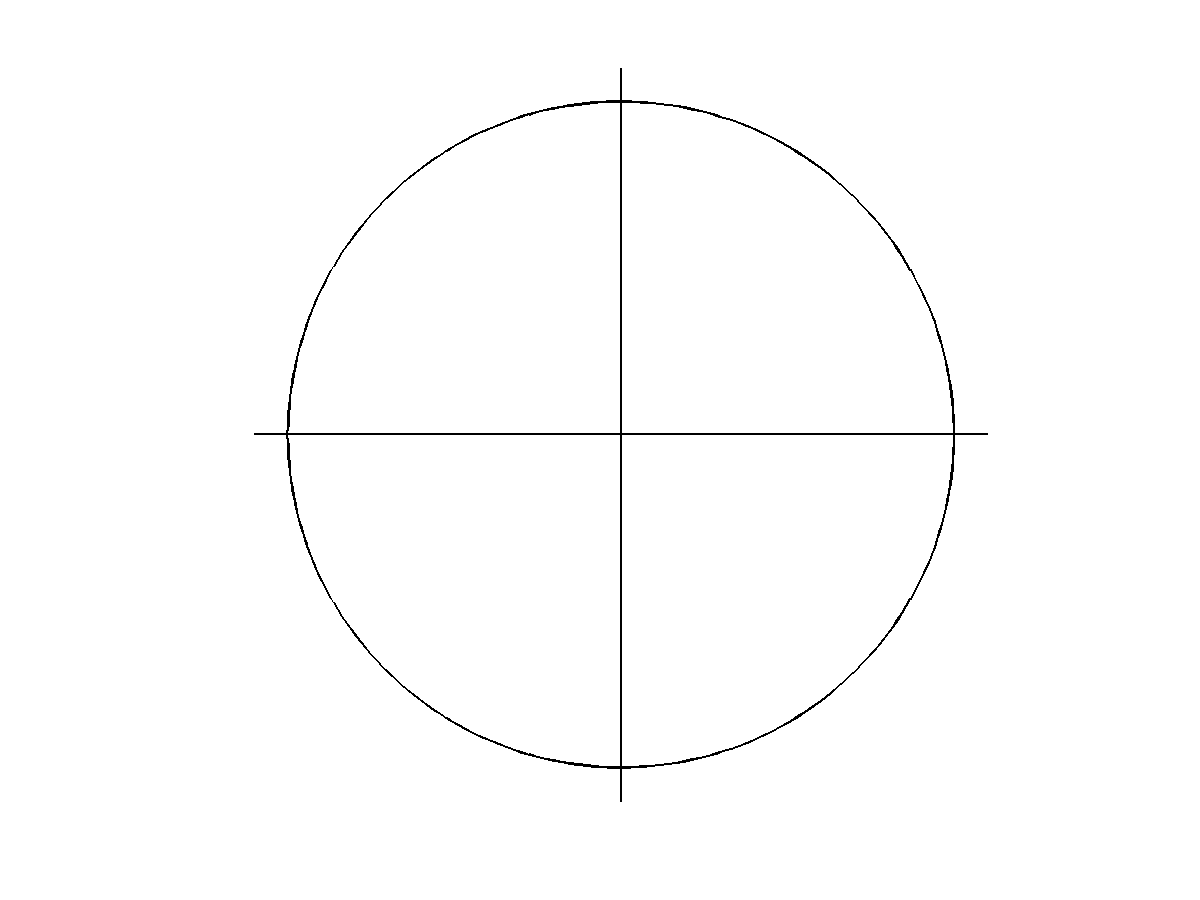
For starters, here is a Matlab code plotting the unit circle and coordinate axes. The axis equal command below is essential to make the circle look like a circle and not like an ellipse.
% Construct angular evaluations points
phi = linspace(0,2*pi,256);
% Create empty figure window
figure(1); clf
% Plot unit circle
plot(cos(phi),sin(phi),’k’,’linewidth’,1)
hold on
% Plot coordinate axes
plot([-1.1 1.1],[0 0],’k’,’linewidth’,1)
plot([0 0],[-1.1 1.1],’k’,’linewidth’,1)
% Axis settings
axis([-1.1 1.1 -1.1 1.1])
axis equal
axis off
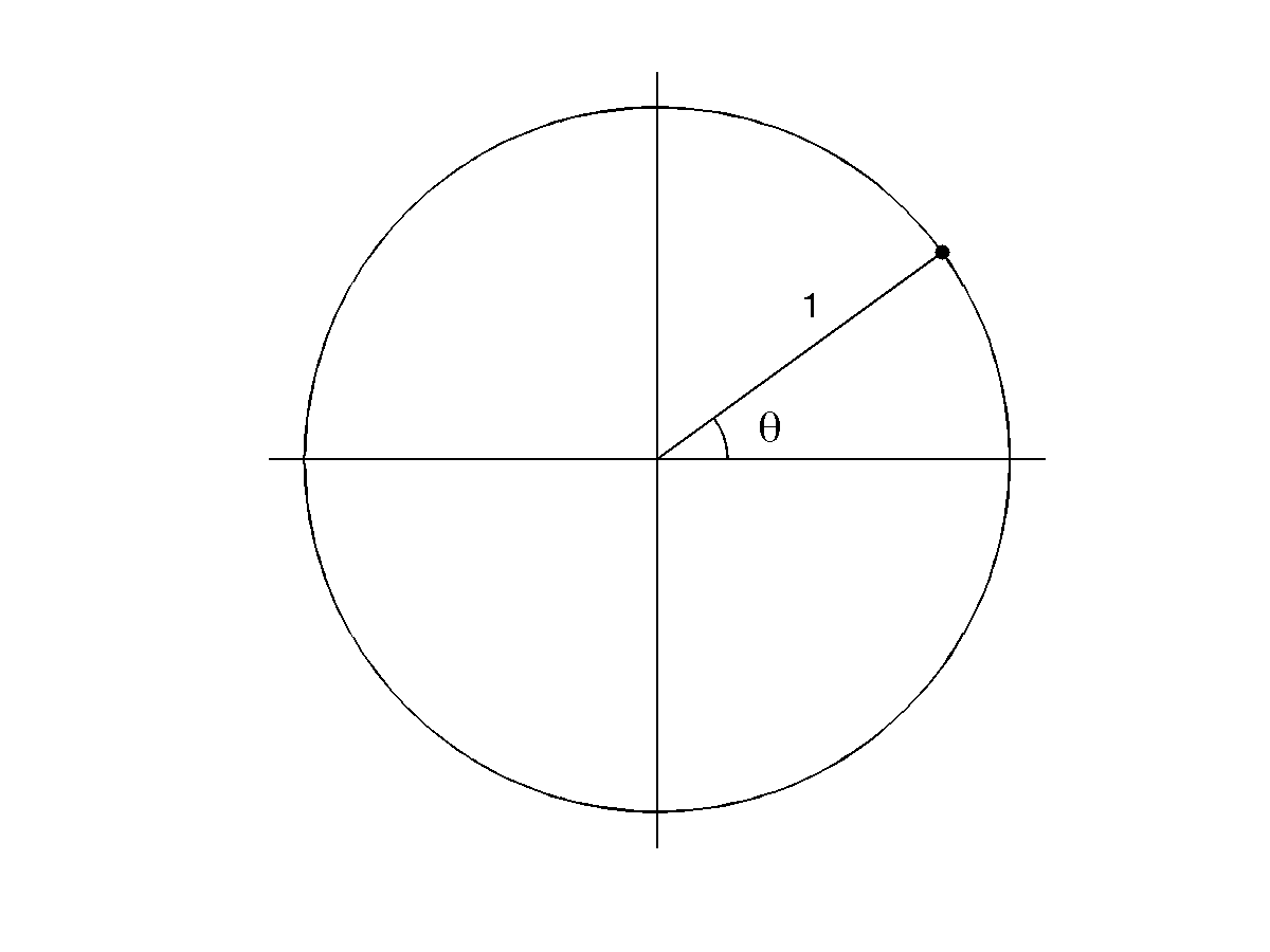
Next we add a point on the unit circle and indicate the angle between the horizontal coordinate axis and the vector with base at the origin and tip at our example point. We call the angle theta. Also, we write the number 1 showing the radius of the unit circle. You can adjust the font size easily.
% Construct angular evaluations points
phi = linspace(0,2*pi,256);
% Create empty figure window
figure(1); clf
% Plot unit circle
plot(cos(phi),sin(phi),’k’,’linewidth’,1)
hold on
% Plot coordinate axes
plot([-1.1 1.1],[0 0],’k’,’linewidth’,1)
plot([0 0],[-1.1 1.1],’k’,’linewidth’,1)
% Choose angle for demonstrating sine and cosine
theta = pi/5;
R = .2;
plot([0 cos(theta)],[0 sin(theta)],’k’,’linewidth’,1)
plot(cos(theta),sin(theta),’k.’,’markersize’,16)
tmp = linspace(0,theta,64);
plot(R*cos(tmp),R*sin(tmp),’k’,’linewidth’,1)
text(1.5*R*cos(theta/2),1.5*R*sin(theta/2),’\theta’,’fontsize’,20)
text(3*R*cos(1.3*theta),3*R*sin(1.3*theta),’1′,’fontsize’,16)
% Axis settings
axis([-1.1 1.1 -1.1 1.1])
axis equal
axis off
% Save image to file
print -dpng sincos2.png
Finally, let’s add sine and cosine using some color.
% Construct angular evaluations points
phi = linspace(0,2*pi,256);
% Create empty figure window
figure(1); clf
% Plot unit circle
plot(cos(phi),sin(phi),’k’,’linewidth’,1)
hold on
% Plot coordinate axes
plot([-1.1 1.1],[0 0],’k’,’linewidth’,1)
plot([0 0],[-1.1 1.1],’k’,’linewidth’,1)
% Choose angle for demonstrating sine and cosine
theta = pi/5;
R = .2;
plot([0 cos(theta)],[0 sin(theta)],’k’,’linewidth’,1)
plot(cos(theta),sin(theta),’k.’,’markersize’,16)
tmp = linspace(0,theta,64);
plot(R*cos(tmp),R*sin(tmp),’k’,’linewidth’,1)
text(1.5*R*cos(theta/2),1.5*R*sin(theta/2),’\theta’,’fontsize’,20)
text(3*R*cos(1.3*theta),3*R*sin(1.3*theta),’1′,’fontsize’,16)
% Show sine and cosine
plot([cos(theta),cos(theta)],[0 sin(theta)],’k–‘,’linewidth’,1)
plot([0,cos(theta)],[0 0],’b’,’linewidth’,2)
plot([0,cos(theta)],[sin(theta) sin(theta)],’k–‘,’linewidth’,1)
plot([0,0],[0 sin(theta)],’r’,’linewidth’,2)
p1 = text(.3,-.1,’cos(\theta)’,’fontsize’,16);
set(p1,’color’,[0 0 1])
p2 = text(-.35,.5*sin(theta),’sin(\theta)’,’fontsize’,16)
set(p2,’color’,[1 0 0])
% Axis settings
axis([-1.1 1.1 -1.1 1.1])
axis equal
axis off
% Save image to file
print -dpng sincos3.png
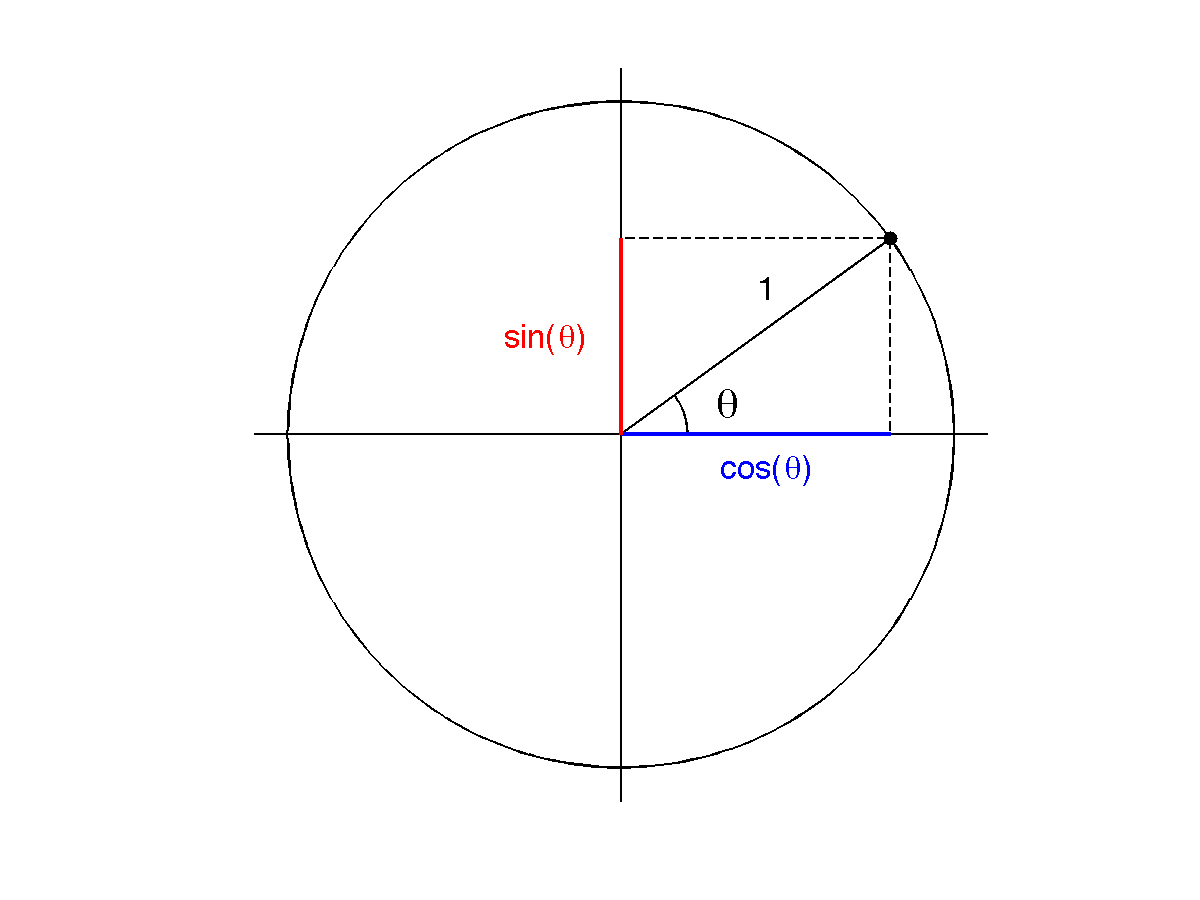
The above color picture is fine for presentations. However, if it will be used in an article, it is better to remove the color and have all the lines and text in black. For this, change the ‘r’ and ‘b’ above into ‘k’. Also, the png file format is pixel-based which is not good for articles. Rather, we need vector graphics and encapsulated postscript (.eps) format. The print command above should be replaced by
print -deps sincos3.eps
(The above command will actually take care of the color issue since print -deps produces black and white images. When you need .eps files with color, use print -depsc.)
Cool, I may stop drawing graphs using latex packages.