Table of Contents

1. Introduction and Background
2. Data
3. Methods and Key Measures
4. Results
5. Discussion
6. Limitations
7. Implications and Conclusions
8. Division of Labor
9. References

Methods and Key Measures

Object Detection and Classification

Manually scanning through thousands of book pages and annotating every printmark takes a lot of time and effort. Given resource and time limitations, the task may become impossible for humans to complete as the page count approaches even larger figures.

Convolutional Neural Networks (CNN), a type of neural network-based computer vision technology, have performed well in a variety of visual identification tasks and yielded results that are on par with or superior to human ability. (He et al., 2015). Faster R-CNN, a popular variant of CNN for object recognition, is a region-based CNN with a two-module architecture that has good accuracy and is fast enough to detect objects in close to real-time (Ren et al., 2015). With Mask R-CNN, which adds segmentation masks to the prior design, faster R-CNN architecture was developed even further (He et al., 2017).  Segmentation masks describe which pixel in the image belongs to which object.

Printmark Detection: Our Approach

Mask R-CNN has already been used for work on Dataset 1, but we wanted to try something else. We decided to utilize the YOLO (You Only Look Once) approach, which Redmon et al. developed in 2016. In contrast to other popular technologies that employ two-step regional proposal methodologies, YOLO is a single-step (or single-pass) network, making it quick by design (Terven & Cordova-Esparza, 2023) Additionally, YOLO was very appealing due to its adaptability to various tasks (detection, classification, etc.), historical performance, and ease of use (Ultralytics, 2023). YOLOv8 by Ultralytics was the most recent version, so we decided to use it.

Printmark Detection: Key Metrics

An important metric in computer vision is average precision (AP), often known as mean average precision (mAP) for multiclass models. This metric is used to assess the model, with values ranging from 0 to 1, with a larger value being better. Simply put, AP is the area under the Precision-Recall curve (see Figure 2.1).

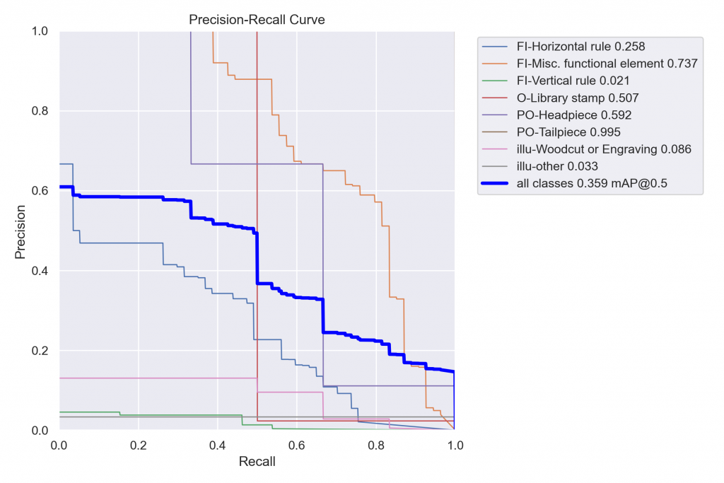
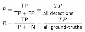
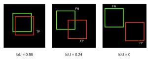
Precision and recall are determined based on true positive (TP), false positive (FP), and false negative (FN) values (see Figure 2.2). Additionally, these values are computed in relation to the Intersection over Union (IoU) threshold (see Figure 2.3). We use mAP@50, where 50 is the IoU threshold, to assess our model’s performance in the printmark detection task.

A model can also be evaluated with a confusion matrix, which compares predicted labels to true labels and in this way summarizes model performance in a single table.  You can find the confusion matrix for our model in the results section.

Printmark Detection: Model Training

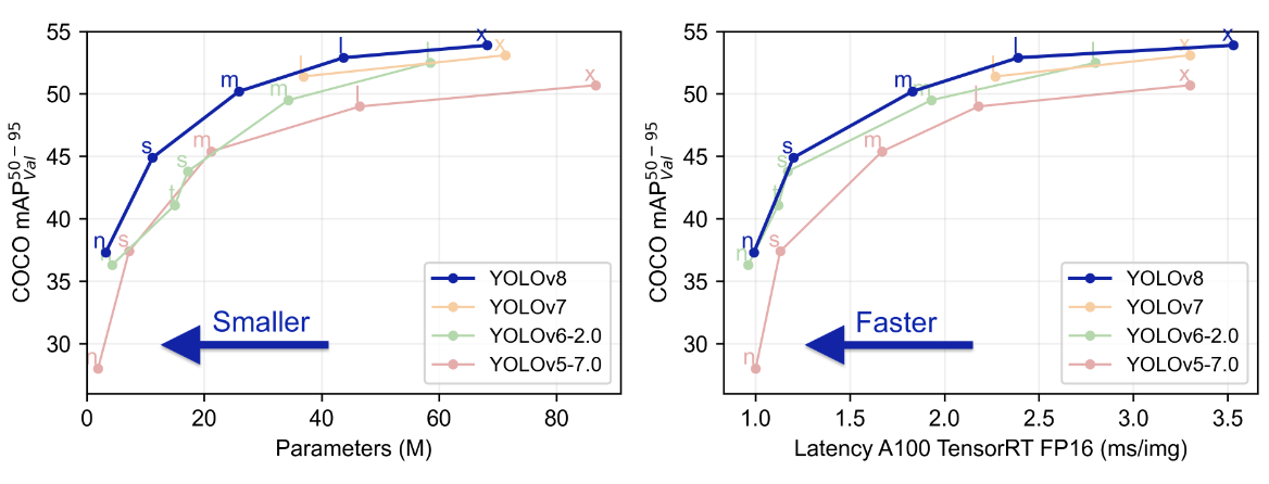
For YOLOv8, Ultralytics offers 5 model sizes (n, s, m, l, x). Figure 2.3 demonstrates that as the model’s parameter set expands,  mAP improves. On the other hand, when parameters increase, mAP improvements become smaller and the model becomes slower and heavier to train. We selected the model size “s” because, according to Figure 2.3, it provides the best boost in performance while remaining quick and reasonably light to train.

Additionally, the pre-trained weights for 128 classes from the Common Objects in Context dataset (COCO128) were used as the basis for training.  The model was then configured to detect only 15 printmarks of interest.

The training process:

1. 1. Annotations from Dataset 1 were transformed into YOLO format.
   2. Dataset 1 images were resized to 640×640.
      • Speeds up training.
      • Same as COCO128.
   3. Class imbalances detected
      • A single book page can contain multiple classes with random counts, which creates problems when balancing training and validation data.
      • Efforts were made to augment the top 5 rarest classes so training and validation data would be more balanced.
      • Augmentation: i) brightness adjustment ii) image sharpening iii) adding Gaussian noise iv) blurring (different from Gaussian) v) adjusting contrast.
   4. A training set of 1723 annotated images was created.
      • Images must contain printmarks, not just text.
   5. A validation set of 237 annotated images was created.
   6. Model training ran for 40 epochs.
      • CPU: 2,6 GHz 6-Core Intel Core i7
      • RAM: 16 GB 2667 MHz DDR4
   7. See results in the result section.

Representation Learning

Images represent a big dimensional space. Just with a 256×256 black and white image we already have 65536 dimensions. Performing learning tasks with such a dimensional space with images is inefficient, because not the whole image brings information that is useful for computations. This is clearly exemplified with video resolution: when you watch a YouTube video, you are able to discern different agents in an image if you watch at 480, 720p or 1080p, but the latter resolutions have more pixels than 480p. This is an example of how we can reduce the dimensionality of an image without losing relevant information.

Taking this example a bit further, we enter the field of Representation Learning, “a paradigm for training machine learning models to transform raw inputs into a form that makes it easier to solve new tasks” (Murphy, 2023). In particular, we focus on using Embed Generation, techniques where we create an image embedding, or an alternative representation of an image that compresses the relevant information in the image into smaller dimensions. This way, we are able to produce alternative representations where we are able to compare automatically how “similar” two images look.

First approach: Neural Networks and PCA

In the fields of Computer Vision and Image Processing, Neural Networks (NNs) have had an incredible impact due to their capabilities in recognizing complex features in images. An example of this is shown in Figure 2.4:

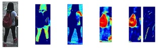
Perhaps one of the most important things that these NNs achieve is learning good feature maps, or in simpler terms, they are good at learning alternative representations of an image: this is so important in fact that many modern object detection architectures dedicate a great amount of resources toward feature maps. For example, one of the most important parts of the YOLOv8 architecture is the Feature Pyramid Network, first presented by Lin et al., 2017. These pyramids are networks wholly dedicated toward obtaining good, lower-dimensional representations of an image for classification tasks, and this is what we wish to do in embedding generation.

An approach toward adapting a NN that has been trained for classification tasks to create embeddings is shown by Masson-Forsythe, 2021. Illustrated with Figure 2.5, a NN trained for a classification task is usually split into two stages: a Feature Extraction stage and a Classification stage. The output of the feature extraction stage is an embedding of the image, which is used by the classification stage to assign a label to a particular image. Hence, it can suffice to remove the last stage to get a network that is capable of embedding generation.

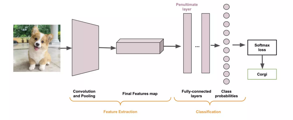
These embeddings would have dimensionality equal to whichever size the last layer of the feature extraction stage has, so it may be helpful to further reduce the dimensionality of the embeddings with some specific dimensionality reduction algorithm. For this work, only Principal Component Analysis (PCA) is considered, both for the aforementioned reduction, as well as for visualization.

The main idea in PCA is to measure how much information can be gathered from each feature in a given dataset, in a way that each feature can be given a weight proportional to its “importance” (James et al., 2021). This way, one can “chop off” the features that give little information for the task at hand. The weight of each feature is given by a metric known as explained variance, which is, intuitively, a measure of how much a change in the feature’s value influences the classification task.

Something that should be noted is that PCA is lossy, which means that after applying a PCA to a dataset, information is lost because it’s just removed. This should be taken into account when analyzing results, particularly if the results are being validated just visually. The information lost usually is not an issue when working with classification, as one can choose an appropriate dimensionality through measuring the explained variance (typically with a plot as a function of number of features), but for visual analysis this is particularly important. If, for example, a dataset’s explained variance is mainly contained within the first 200 dimensions, too much information may be lost when doing a PCA to 2 dimensions for visualization, so they should be taken with a grain of salt.

Second approach: NORPPA

NORPPA was originally designed by Nepovinnykh et al., 2022 as a content-based image recognition (CBIR) system to operate on images of ringed seals. The CBIR approach requires a database of labeled images, where a given image can then be identified by its content as being similar to one of the labeled images. This matching process can be done one-to-one or one-to-many, depending on whether the system determines the label for the query image by selecting the label from the closest image in the database or by using more complex techniques to match an image to several images and obtain a label through one-to-many matching. Alternatively, if the database lacks labels, the same algorithms can be employed for clustering as the feature vectors of images within the database are grouped together in feature space for images with the same label while they are far apart for those with different labels.

NORPPA implements Fisher Vector, a technique that takes local characteristics of an image, combines them into a concise feature vector, and represents the contents of the image. To compile features from local patches, it employs a Gaussian Mixture Model (GMM) for clustering. Once the clusters have been formed, a visual word dictionary (codebook) is created by Fisher Vector using the GMM’s findings. Images are then translated into vectors using this dictionary. The shortcoming of this method is the Fisher Vectors’ dimensionality, which is given by (2D+1)*K, where D represents the descriptor’s dimensionality (local characteristics) and K represents the quantity of components (clusters) in GMM. For descriptors with 64 dimensions and a low cluster quantity of 256, the resulting Fisher Vector dimensionality is (2*64+1)*256 = 33024, which is computationally impractical. As a result, the dimensionality of vectors is generally decreased further using PCA.

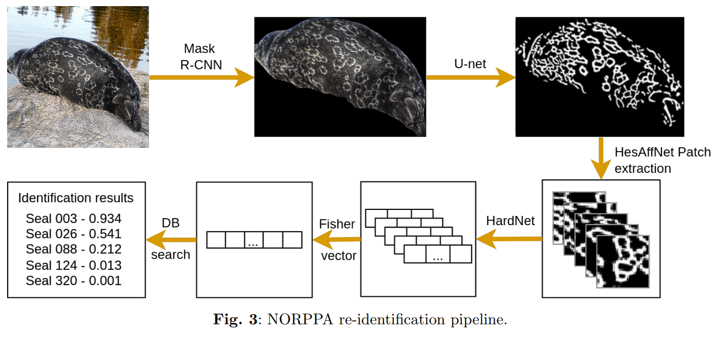
NORPPA’s initial step is to generate a codebook and fisher vectors for the pictures in the database. Initially, HesAffNet is used to extract good patches from the images, which are then passed to HardNet to produce local descriptors. Next, PCA is performed on these descriptors to uncorrelate them and minimize their dimensionality, which eases the construction of fisher vectors. A codebook is then formed by using GMM, as previously described, and kept for future use. Then, fisher vectors are produced for each picture in the database using the codebook and local features from an image. Finally, KPCA is applied on the resulting fisher vectors to reduce their dimensionality. Note that the process is entirely unsupervised, allowing for the approach to be employed for clustering.

Once the codebook and fisher vectors were created for the images in the database, the system is utilized to match query images with those from the database. The pipeline is close to the one described above. First, suitable patches are extracted through HesAffNet, which are then passed to HardNet to produce embeddings. The embeddings are encoded through trained PCA to further reduce the dimensionality. by utilizing the codebook that was generated for the database and the local descriptors acquired from the query image, a fisher vector is constructed which is then further dimensionally reduced through trained KPCA. It is then employed to match the query image to the images from the database. The general pipeline is depicted in Figure 2.6.

The clustering of headpieces and initials in the current project can also use the same pipeline. If the number of images is small (up to 10k), fisher vectors can be created by constructing a database using the previously described method. For larger datasets, a random subset of images can be used to form a database, then fisher vectors can be generated for other images as query input. The resulting fisher vectors can be clustered using OPTICS or other similar methods as explained in the following section.

NORPPA has several advantages. The method is generally applicable to any type of images, not only ringed seal patterns, as HardNet, used for generating local features, was trained on a large dataset of patches from real-world images. Another benefit of the technique is that it can be used to construct feature vectors that combine features from both the headpiece and the initial from a book page. To do so, one should create a new codebook, which applies GMM on features from patches from both initials and headpieces. The fisher vectors can then be formed by utilizing the codebook and local features from the initial and the headpiece from a page. However, NORPPA has some drawbacks. The usage of fisher vectors requires a lot of RAM for forming a database. Further, the method is computationally complex as several hundreds of patches are passed through HardNet (a convolutional neural network) for one image.

Unfortunately, during the project we did not have time to test embeddings generated by NORPPA, so it may be a good starting point for future groups. You can find a guide on how to use NORPPA for the project here.

Image Clustering: OPTICS

After producing embeddings with a NN and reducing their dimensionality with PCA, one can apply a wide array of clustering techniques on images such as k-means and DBSCAN. A comparison between many such techniques is available from the scikit-learn documentation, available here. The technique explored in this work is Ordering Points To Identify The Clustering Structure (OPTICS), developed by Ankerst et al., 1999, which can be seen as an extension or generalization over DBSCAN.

A key characteristic of the dataset in the current work is that the distribution of printers represented in the works is not uniform, so different clusters will most likely have a different number of members. Because of this, purely distance-based algorithms like k-means are not a good fit for finding clusters, as they will group together different observations even though they may be far away. Due to this, one should opt to use density-based clustering algorithms. OPTICS is one such algorithm.

OPTICS takes two main hyperparameters: a maximum distance ε and a minimum number of observations per cluster MinPts. At a high level, the algorithm first looks for the “cores” of the clusters by the amount of objects that they have close by, discarding the ones that have a distance bigger than ε. Then, a cluster is defined if there are at least MinPts objects close to the core. Objects that do not fit these conditions are labeled as noise and do not belong to any cluster.

Metadata Analysis

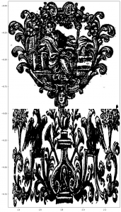
The main problem of the analysis of the clustered Dataset 1 is the missing comprehensibility. Figure 2.7 shows cluster number 9 in which ornaments seeming to be completely different were grouped. The shapes and the content don’t match and it’s not understandable why the algorithm clustered those two together. Probably, features such as size, outline and shapes have an important influence, but as cluster 9 exemplifies, the algorithm probably used many more unknown features. Given that an analysis on that basis would be more guesswork than a structured examination, we focused on the only other information available: The metadata records. The small number of meaningful clusters, missing benchmarks and the many gaps in the data additionally suggest a qualitative, exploratory approach.

For each work in a meaningful cluster containing different ECCO ids (meaning that the ornaments clustered derived from different books or pamphlets), the following metadata was collected:

• • About the works: Publication data, publication place, publication country,
  • About each actor involved: Actor name, actor id, actor role.

An examination of the metadata should be able to answer whether the works in the same cluster have the same actors, e.g. publisher, or whether they were published in the same place or time. The results of this analysis are not as expressive as the direct comparison of printer information, but, if those printer information are not available, the results can be indicative whether it is possible that the works were printed by the same person. If the works were published in two different towns or if the time gap is relatively huge, the probability that the work was printed by the same printer is unlikely. Additionally, if two works were published or authored by the same person, the probability that the same printer may have been mandated to print both works is higher, although not necessary.

< Previous section: Data | Next section: Results >