Table of Contents

1. Introduction and Background
2. Data
3. Methods and Key Measures
4. Results
5. Discussion
6. Limitations
7. Implications and Conclusions
8. Division of Labor
9. References

Results

Printmark detection: YOLOv8

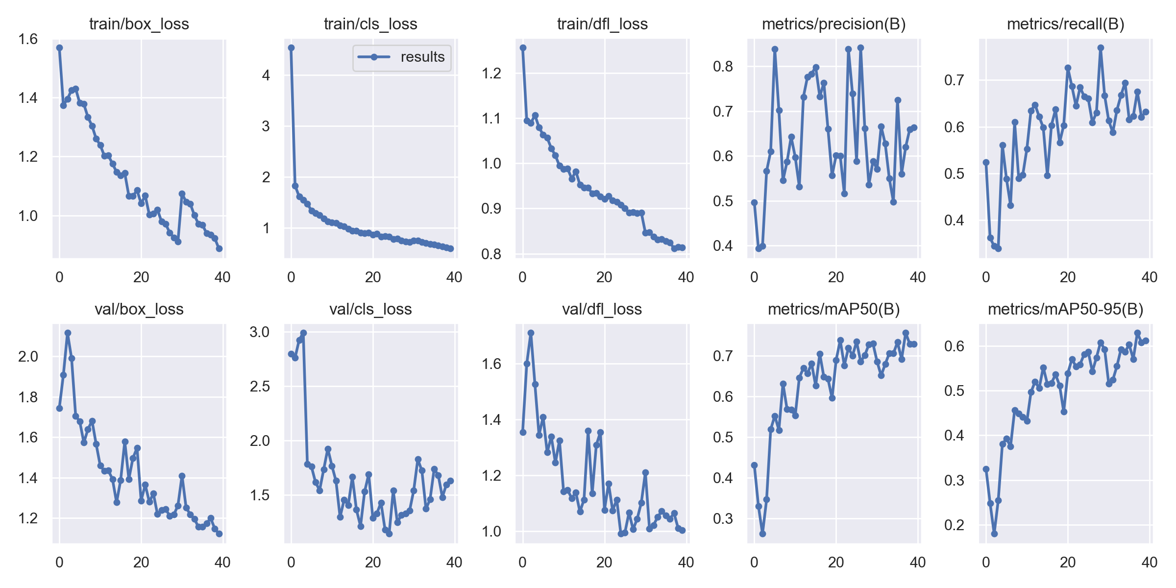
Here are the results of our YOLOv8 training and validation. Figure 3.1 shows the entire 40-epoch run. The model managed to learn from data and the mAP steadily rose over time.

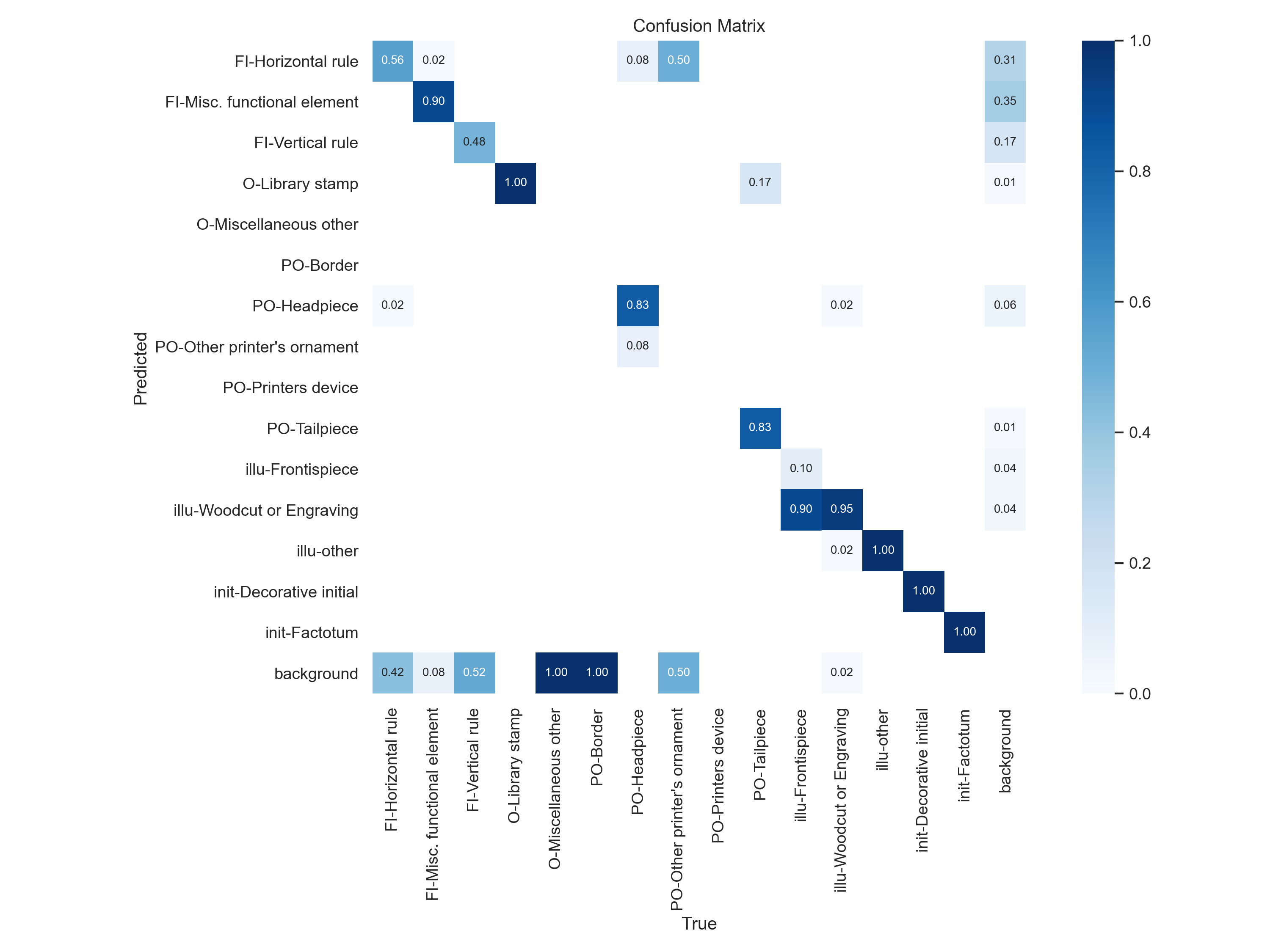
In Figure 3.2 the confusion matrix is shown. The model performed well in detecting the following 8 classes: FI-Misc. functional element, O-Library stamp, PO-Headpiece, PO-Tailpiece, illu-Woodcut or Engraving, illu-other, init-Decorative initial, init-Factotum. Notable is the complete absence of detections of PO-Printer’s device class.

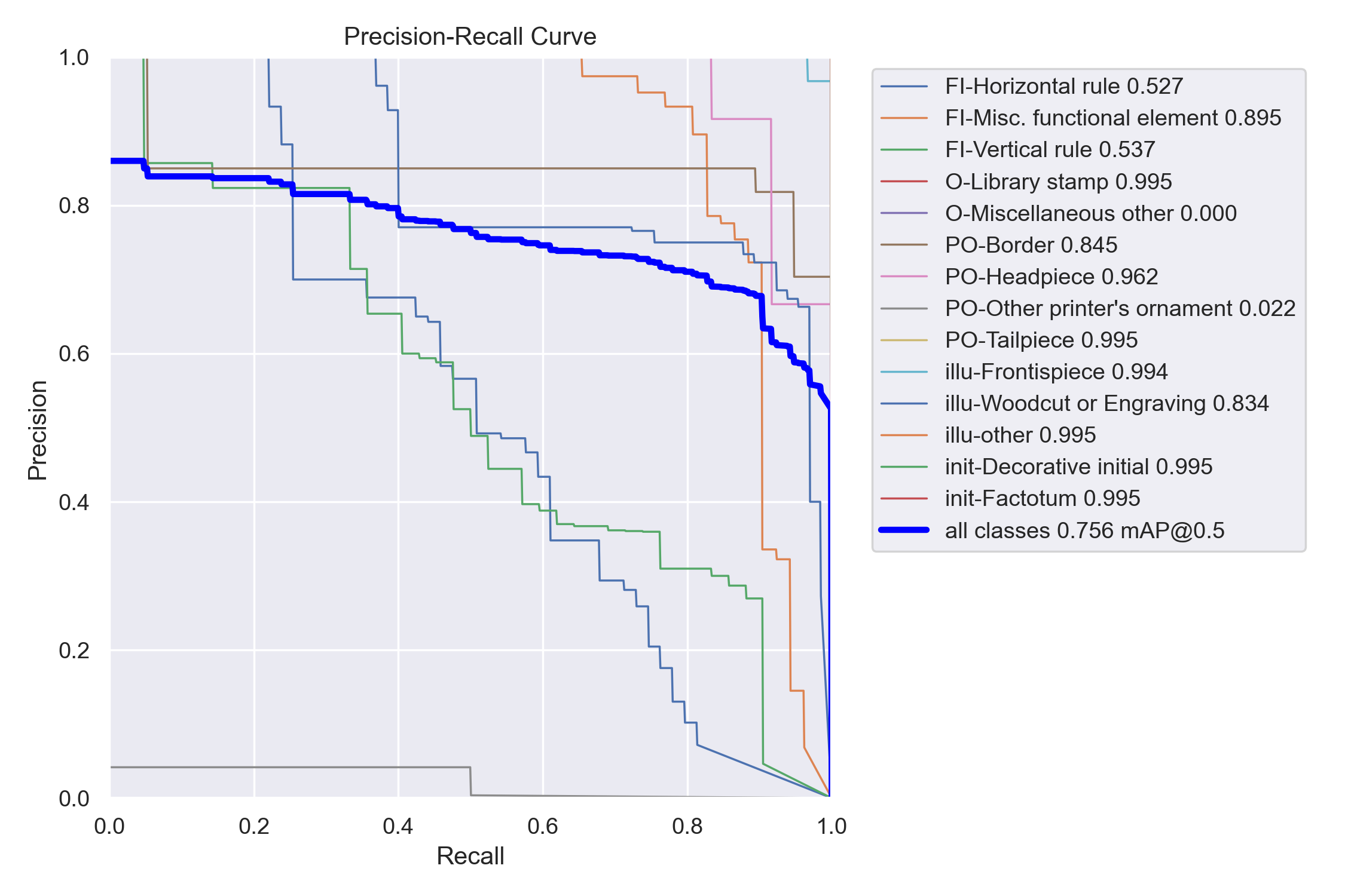
Our model managed to achieve mAP@0.5 of 0.756. This and all the individual class APs can be seen in Figure 3.3.

Figures 3.4 and 3.5 demonstrate the annotated ground truths versus model predictions in a batch of 16 randomly selected pages. Predictions come also with a confidence score between 0 and 1.

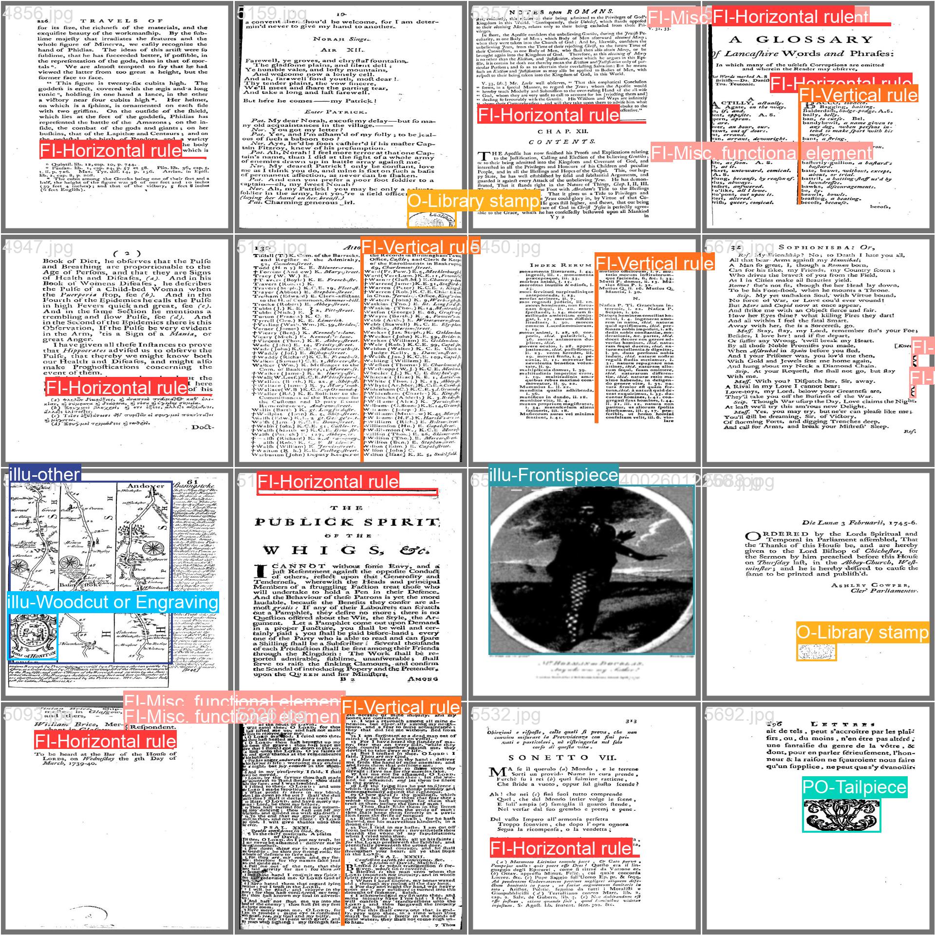
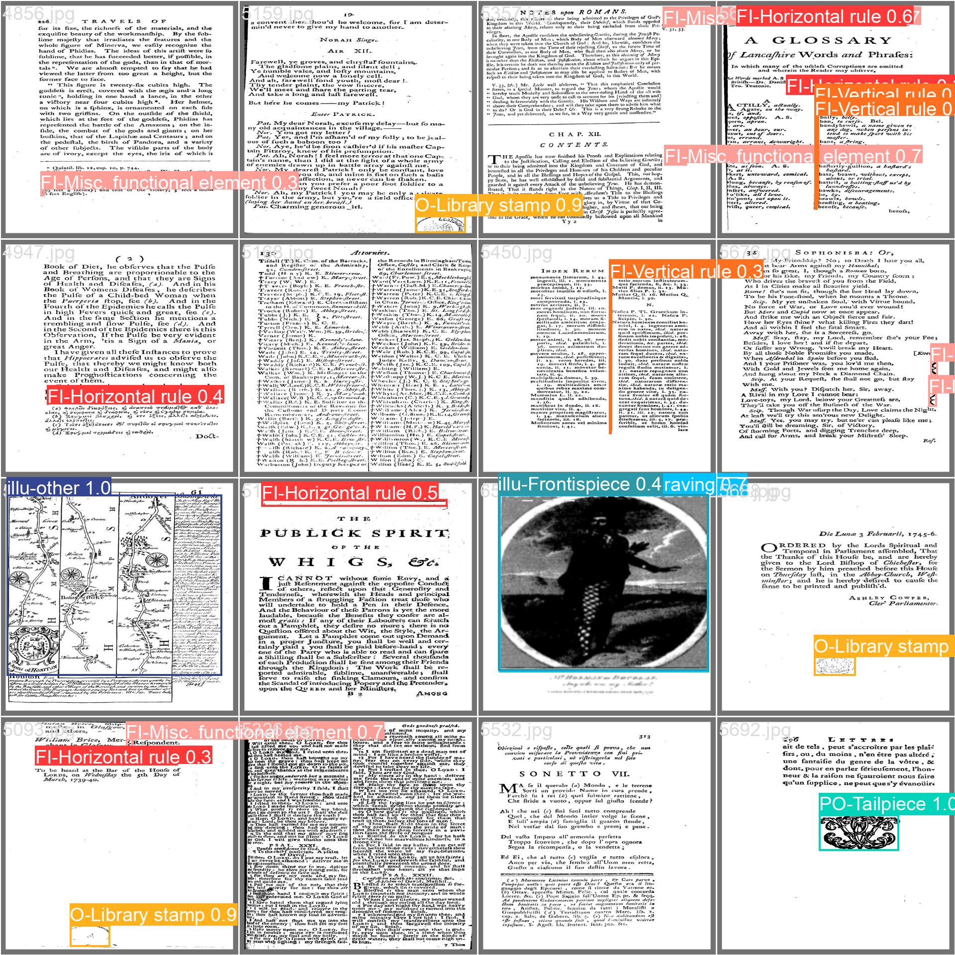
Image Clustering: Embeddings with ResNet50

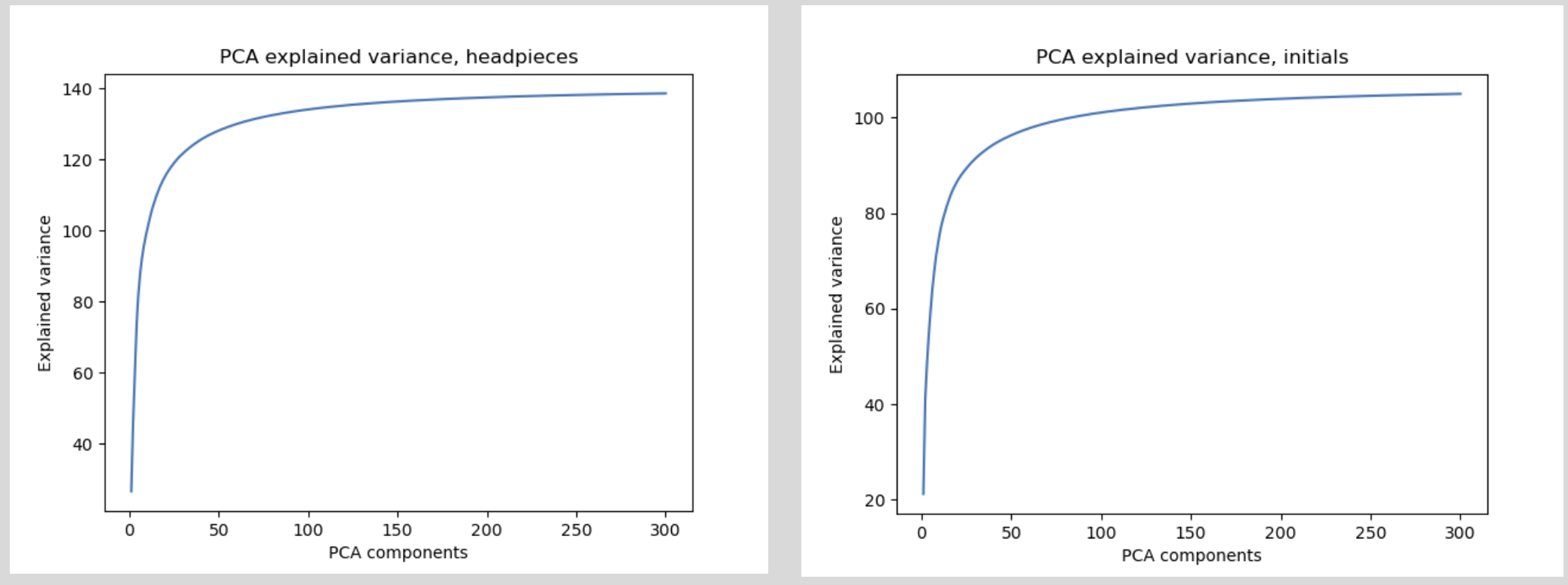
For this work, we used a pre-trained ResNet50 NN provided by PyTorch, following the approach presented by Masson-Forsythe, 2021. The embeddings generated with this NN are 2048-dimensional, so we used PCA to see if we could reduce this space further. The explained variance on embeddings generated separately for headpieces and initials is shown on Figure 3.6:

After reducing the embeddings to 300 dimensions, we can look at different clusters on a test dataset to evaluate the performance of the approach. The clusters were generated using OPTICS with a cosine distance metric, with a maximum distance of 0.8 and a minimum of 2 objects per cluster. First we look at the images that were labeled as noise in the headpiece and initial groups in Figure 3.7:

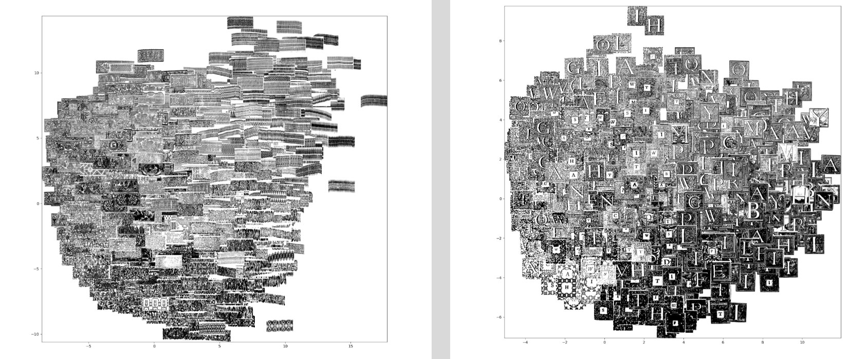
We can see that there are many images that were labeled as noise. With this approach and after hyperparameter tuning, the biggest proportion of the datasets (headpieces and initials) that we could cluster was around 60%. Resolution and/or image size seemed to affect this result, although bigger images imply a bigger computational bottleneck.

Some results of using the proposed clustering approach on the headpieces are shown on Figure 3.8:

 

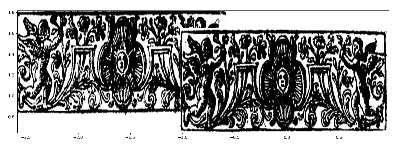
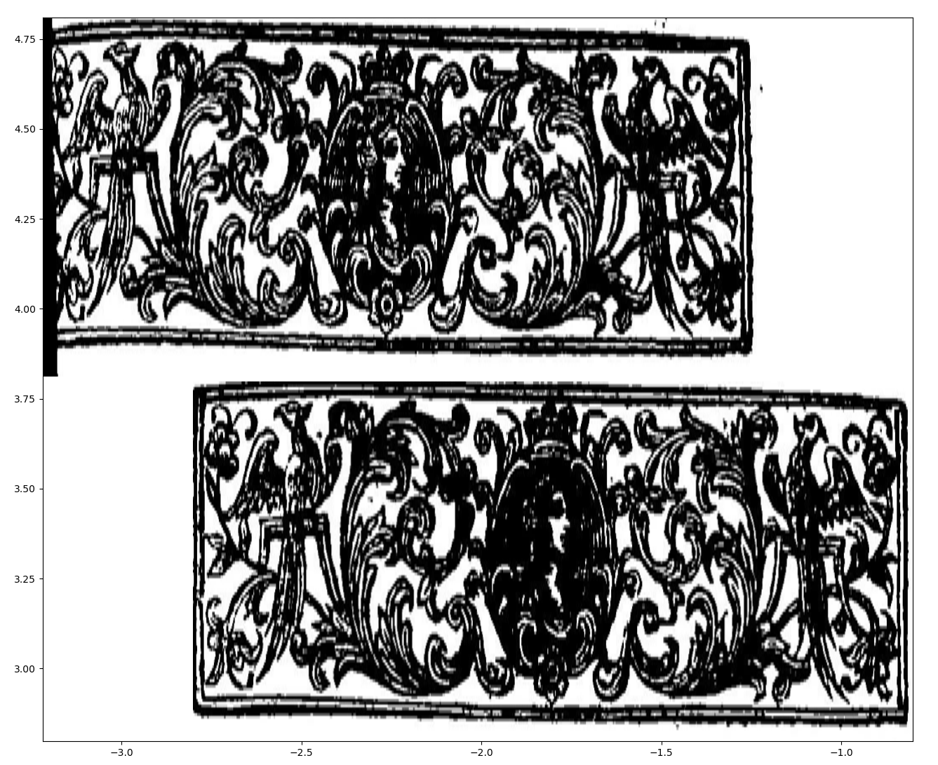
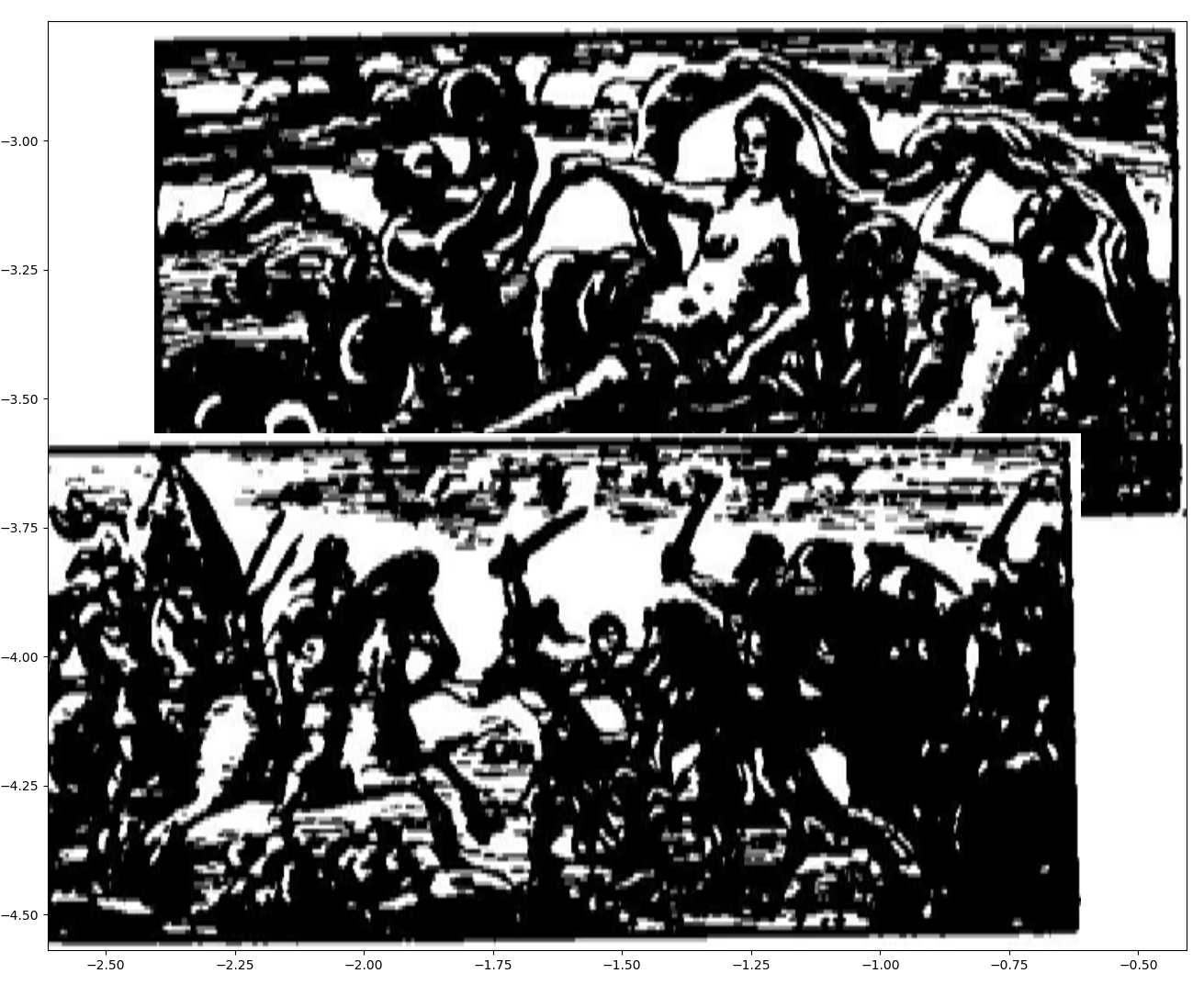
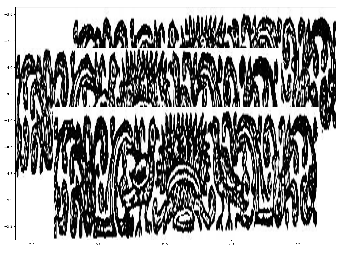
Figure 3.8: Clustering headpieces using embeddings generated from a pre-trained ResNet50 neural network.

The observed clusters hold a high degree of similarity, and the pieces need not be the same. For example, the Tonson headpiece cluster 250 observed on Figure 3.8.c puts together two headpieces that are stylistically similar, though the illustrations are quite different.

Then, some clusters obtained on the initials are shown on Figure 3.9:

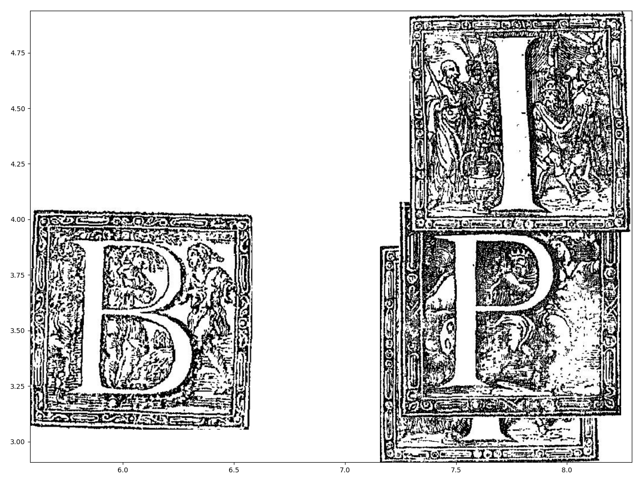
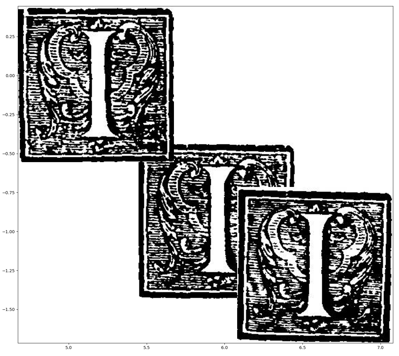
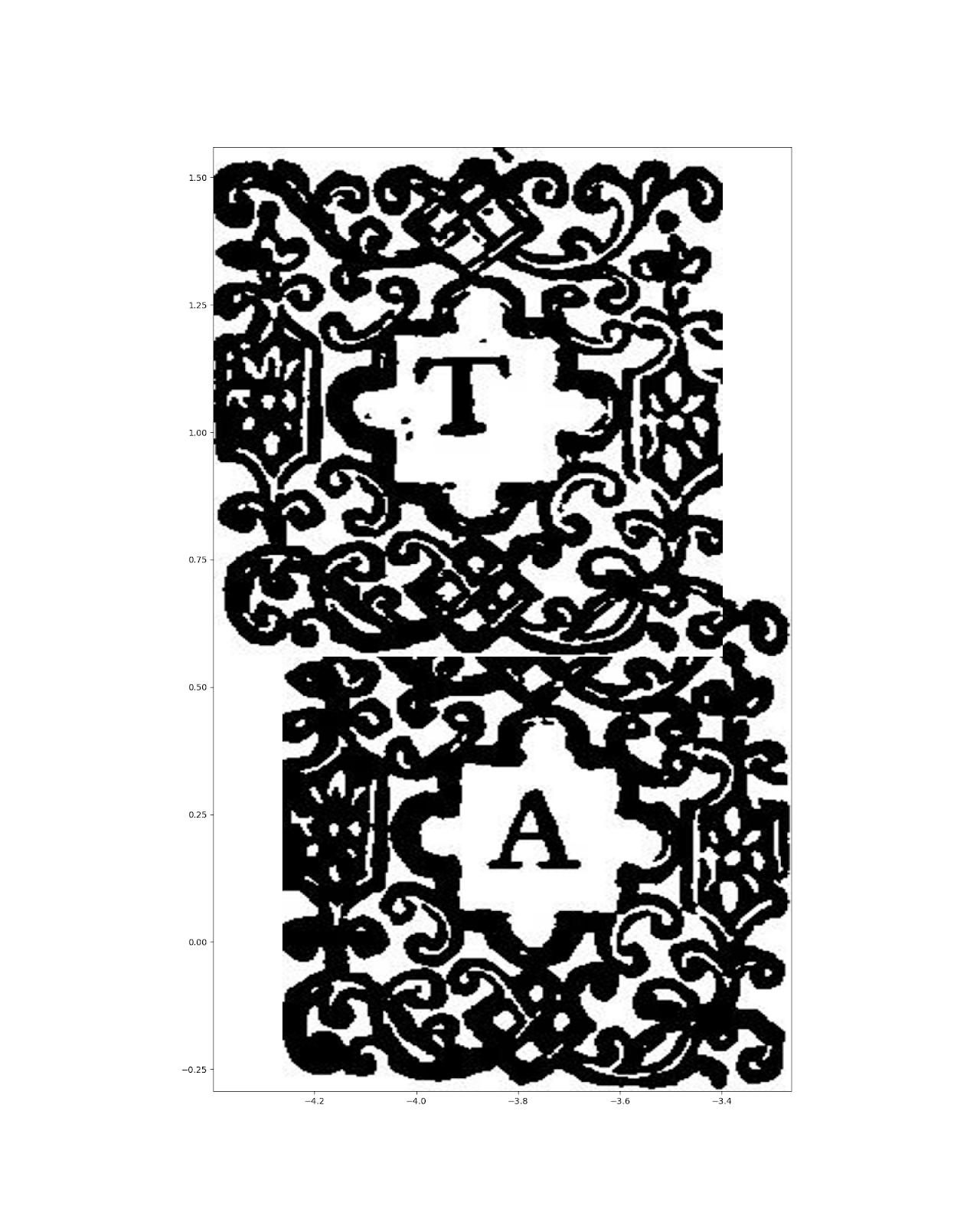
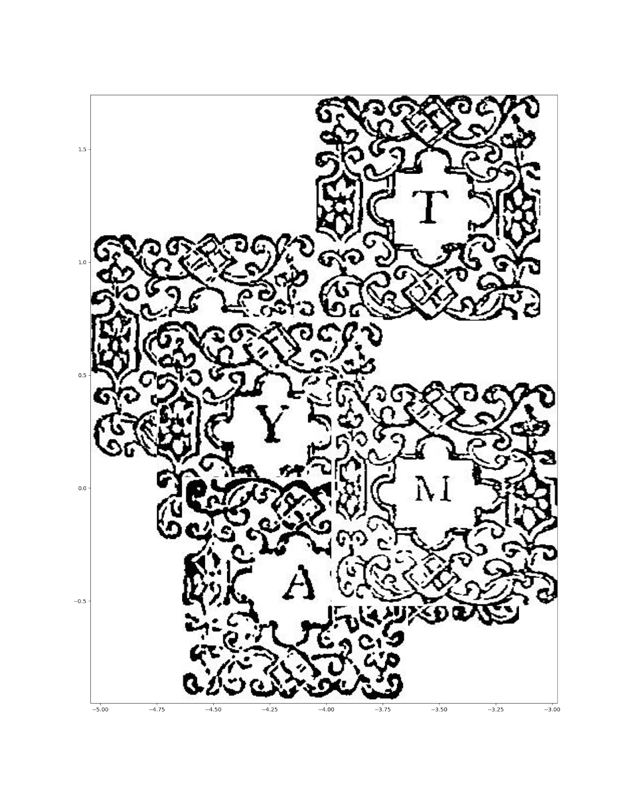
Figure 3.9: Clustering initials using embeddings generated from a pre-trained ResNet50 neural network.

Similarly to the headpieces, with the method we can capture similarity quite well on the Tonson dataset’s initials. Letters themselves do not seem to have much bearing on the clusters , and Figure 3.9.a shows quite a diverse cluster of initials that share similar styles.

Dataset 1: Description of Clusters

The clustering using YOLO resulted in 469 clusters, from which only 24 were meaningful. In many of the not meaningful clusters, only parts of images were used for the clustering, resulting in odd results as can be seen in Figure 3.10.

Overall, 16 of the 24 clusters contained at least one work for which the information about the printer is provided in the metadata record. The clusters 3, 5, 7, 9, 17, 34, 38, 39 do not contain any information about the printer and are not considered in the following paragraph.

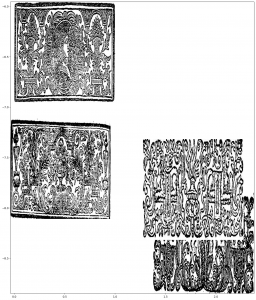
The cluster 0 and 2 contain more than one printer id which diverge from each other. Cluster 0 contains many ornaments of the same book which is generally a sign for the algorithm recognizing ornaments with a similar style. The clustering of ornaments from different printers on the other hand indicates that the clustering is not fine-grained enough because ornaments containing common signs and styles are clustered together. Moreover, obviously same ornaments like the box shown in the clusters 29, 30, 31, 32, 33, 35, see Figure 3.11, are divided in several clusters. Probably, the feature size and rotation may have prevented the clustering into one cluster, but those two features do not explain why the cluster 30 and 31 are not one bigger cluster.

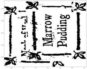
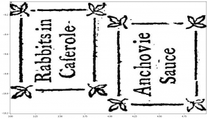
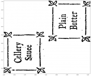
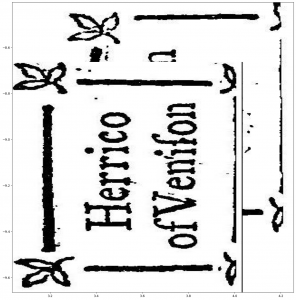
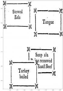
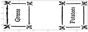
Figure 3.11: Clusters with the same ornament.

Results of the metadata analysis

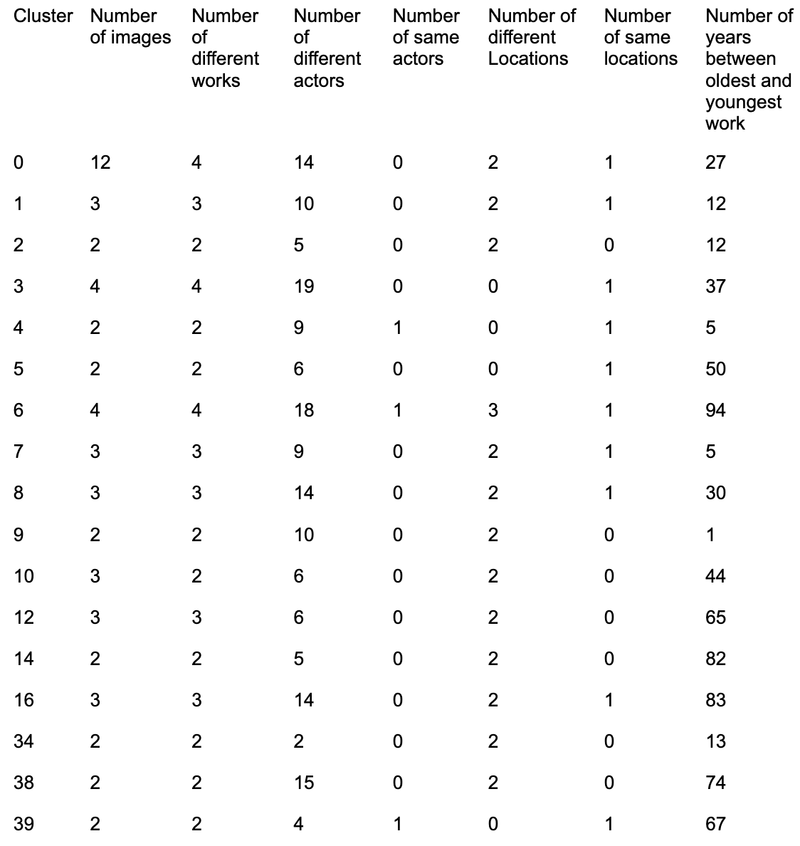
Table 1 shows the results of the metadata analysis. The general findings of the indicative evidence is tending towards a negative result for our purpose of identifying printers. Many works were published in different towns and if not, they were published in London which is, as explained in the section about the data, the location where by far the most works were published and therefore London as location is not as expressive as other locations would have been. For 9 clusters, the time gap was bigger than 30 years, which is for a device made out of wood and regularly used, a relatively large time span. Only in 3 clusters, the same actors were involved in the publication cycle. For some of the clusters, e.g. cluster 34, the number of involved actors seems to be quite low, indicating that metadata about involved actors may be missing. The clusters with intersecting actors are examined further in the following paragraphs.

In cluster 4, two ornaments of works published by William Taylor within 5 years were clustered together. One of the works was printed by John Darby, thus it could be the case that the other work was also printed by John Darby. On the other hand, the ornaments , as can be seen in Figure 3.12, have a similar style although they are quite different. It could also be that the style was caused by a request of the publisher. The blurred borders between publisher and printer complicates the allocation of responsibilities. Additionally, if size and shape are indeed important parameters for the clustering, the setting of ornaments and the design of the page could lead to publisher specific dimensions and those may have influenced the grouping.

Two works were also published by the same publisher in cluster 6, see Figure 3.13. Again, this could be a hint that the works were also printed by the same printer, but no printer information is available for one of the works. Both works were printed and published in Dublin. The other two works in the cluster were published in Scotland and London which leads to the conclusion that those were not printed by the same printer. Again, specific dimensions and style-specific aspects may have led to the clustering, but it is interesting that the four works were clustered into one cluster and not into two, because the two ornaments at the left side seem to be much more similar than the other two ornaments.

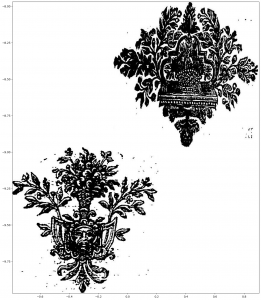
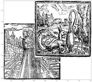
Figure 3.14 shows cluster 39 in which two ornaments of works from the same author but different publishers were grouped together. Interestingly, both works broach the issue of Æsop’s fables and the ornaments have a very similar style and show a differentiated picture of a scene of the fable. Overall, the three clusters indicate that the clustering takes style-specific, rare parameters into account. Thus, the clustering may not be reliable enough for a printer identification, but can maybe be used for other purposes like the detection and grouping of rare ornaments and be interesting for historic scholars working on design and style of ornaments.

 

< Previous section: Methods and Key Measures | Next Section: Discussion >