There is limited information out there about how to do visualisations with VisIt and ghost zones, so I decided I had to put it out myself. But first, some context.
VisIt handles many different file formats for the source data, but many of them are specialised or require one to do a lot of ‘post processing’, either using VisIt’s powerful python API or by mangling together expressions in the GUI. Alternatively, one can tell VisIt how the data is structured by writing it to a file using the Silo library. This writes data using the HDF5 format (although Silo can also handle others).
When the data come from one machine, that’s all well and good. But when the dataset comes from multiple machines, often there are ‘haloes’ or ‘ghost zones’ where the data on each node overlaps. When doing domain decomposed simulations with finite difference equations, depending on the stencil, one needs to know values beyond the boundary of the domain being simulated. This is because the ‘next’ value at a point depends on the value of the neighbouring points, and sometimes those points are being simulated by a different processor:
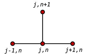
Finite difference stencil. Public domain image [source]
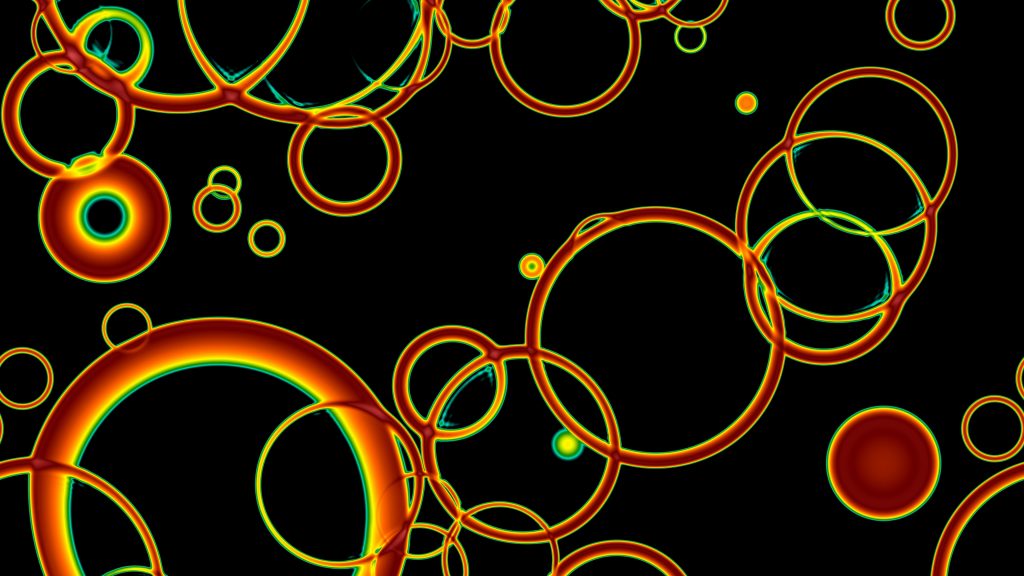
When writing these overlapping zones using Silo, each node writes its own file, and then a ‘root’ file is made by one node that stitches them all together. This is called ‘PMPIO’ (poor man’s parallel I/O) in the Silo library parlance. I like it because it makes relatively few assumptions on the parallelisation or available libraries on the machine, but it does put a strain on the parallel filesystem receiving the data; this can be mitigated somewhat by letting only one node at a time writes its file.Anyway, once you’ve got all your data written and stitched together, you can put it together and get something that looks like this:

The same data with ghost zones from the four nodes that have each done part of the computation.
Uh oh! This picture is the result of a simulation over four cores, and where the simulations on those four cores overlap, the transparent colour is darker! How do we fix it?
How not to fix it
You might at first think – as I did – “ok, no problem, just remove the halo data and write the files. VisIt will stitch it together and it will look nice”. No, VisIt will not stitch it together:

The same data without any ghost zones at all.
One has to tell VisIt something more about the data it is reading, before it will get the hint.
Data offsets: the absolute bare minimum
Now we come to the point of this blog post: how does one fix this without wading through piles of API stuff and writing stuff blindly? I googled a bit and turned up some discussions, and there is some documentation of how to implement ghost zones in the official “Getting data into VisIt” guide available here; the Silo API is fully but opaquely documented in its user guide available here. There’s also an accompanying example source file, ghostzonesinfile.c, extracts of which are in main guide. But that conflates mesh extents and offsets, and it has absolutely no comments so for a novice it may not be immediately clear what needs to be done to get your ghost zones adequately represented.
Assuming you are using a rectilinear mesh with periodic boundary conditions, distributed over several nodes, you need just one thing: the offsets, telling VisIt how much of the data at each node should be treated as ‘ghost’ data.
Despite what the content of ghostzonesinfile.c would suggest, you do not need:
- The extents of your mesh on each node – these data are redundant anyway, as you give the mesh extents implicitly in the quadmesh specification.
- The data extents of any variables you are using – VisIt can surely figure these out for itself.
Hence, because it seems to me that ghostzonesinfile.c is much more complicated than necessary, I wanted to make a post about this.
Setting the offsets
First, I make a DBoptlist:
DBoptlist *dboptlist = NULL;
dboptlist = DBMakeOptlist(1);
Then for my particular case I reverse the order in which data are stored, just because of how I do things. I’m including this here, as it might be useful for someone else who’s trying to figure out why their data look messed up:
const int row_major = DB_ROWMAJOR;
DBAddOption(dboptlist, DBOPT_MAJORORDER, &row_major);
Then I create two arrays with the offsets for the current processor:
int hi_offset[3], lo_offset[3];
These arrays (in my case reversed: {z, y, x}) will each contain how many lattice sites to treat as ‘overlap’ on each end of the domain.
My code is domain decomposed in the x– and y-directions, with each node getting the full length of the z-direction. I have nx nodes in the x-direction, and ny nodes in the y-direction. First, I work out where in this grid the node running the code (identified with MPI rank p.rank) is located:
int this_posx = p.rank % nx;
int this_posy = (p.rank - this_posx)/nx;
Then I set the offsets. As there’s no haloing in the z-direction, the offsets there are zero.
// z-dir
lo_offset[0] = 0;
hi_offset[0] = 0;
For the other two directions there are haloes/ghost zones. For some reason, there needs to be an overlap of exactly one for the resulting isosurface to look smooth, so I choose to keep the high halo entry, and tell Silo the lower one is to be ignored, except on nodes on the high end of the y-direction domain decomposition, where there’s no need for an offset because there’s no neighbouring node:
// y-dir
lo_offset[1] = 0;
if(this_posy == ny - 1) {
  hi_offset[1] = 0;
} else {
  hi_offset[1] = 1;
}
Finally, the x-direction looks pretty much the same.
lo_offset[2] = 0;
if(this_posx == nx - 1) {
  hi_offset[2] = 0;
} else {
  hi_offset[2] = 1;
}
Note that, although the silo documentation linked above says that the high offsets are ‘zero-based’, to be specific a value of zero here means that no offset is present. This was a bit ambiguous, but is clear from reading ghostzonesinfile.c.
Then one adds these offsets to the DBoptlist:
DBAddOption(dboptlist, DBOPT_HI_OFFSET, (void *)hi_offset);
DBAddOption(dboptlist, DBOPT_LO_OFFSET, (void *)lo_offset);
Then one simply calls DBPutQuadmesh, DBPutQuadvar1 and DBPutQuadvar with the dboptlist, for example:
DBPutQuadmesh(dbfile, "quadmesh", NULL, mesh, meshsize, 3,
DB_DOUBLE, DB_COLLINEAR, dboptlist);
I just gave the offsets to everything, on each node, and it worked. When it came to calling DBPutMultimesh and DBPutMultivar on the ‘root’ node, I didn’t specify anything. It Just Worked!
Final caveats
Annoyingly, older versions of both Silo and VisIt will not work with this method of representing ghost zones. If you think you’ve done everything correctly but aren’t seeing anything, check they are both up to date. In the case of Silo, things may compile properly, and linking will be okay unless you are trying to link against a different version than that for which you used the header files, but at runtime when saving your data you may see error messages like:
DBAddOption: Invalid argument: optlist nopts
If you see messages like this, check you are using the most recent version of Silo.
 Visiting graduate student Daniel Cutting was back in Helsinki for a week and in that time attended the Fall Meeting and Christmas Dinner of our Doctoral Programme in Particle Physics and Universe Sciences. He was invited to give a presentation but, rather than speaking about his research–which includes one paper based partially on work done in Helsinki with Helsinki researchers–Daniel gave a rather different kind of talk. Here is what he has to say:


.jpg)