
This week’s topic has been analyses, focusing on network analysis in GIS. We have read and discussed different topics in network analysis such as usage, terminology, algorithms, and functions. The most known and used algorithm in network analysis is called Dijkstra’s algorithm which is based on the mathematical graph theory.
In this week’s assignment, the task was to get familiar with the network analysis methods and concepts and use different tools and functions to solve routing problems as well as to calculate distances to nearby objects. To complete this exercise, I have used different queries, tools, and functions as well as observed statistics and combined different databases and layers.
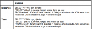
The first part of the assignment was to create the shortest bicycle route from Porthania to Kumpula campus using the Dijkstra algorithm. I calculated both the distance, as well as the time of travel from Porthania to Kumpula campus. This analysis was made with queries which are listed below in table 1.
Table 1. The table lists the queries I used when creating the shortest route from Porthania to Kumpula campus. The algorithm is based on Dijkstra’s algorithm.
I did the same analysis twice, in the second analysis, I used a different function. The second function I used, shortest path, is a QGIS providing network analysis function. To perform the shortest path analysis, the start and end vertex need to be chosen from the map, I chose Porthania as the start vertex and the end vertex as Kumpula. I also added a few variables, such as the digitization direction of the roads which affected the outcome of the analysis.
The routes that the two analyses gave were quite identical except for one minor difference. The start of the route differed. The first analysis route started from the Yliopistonkatu and went along the Fabianinkatu to Kajsaniemikatu. The second analysis route also started from the Yliopistonkatu but went along the Vuorikatu instead of Fabianinkatu to Kajsaniemikatu. This was the only noticeable difference between the two analyses.
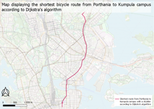
Picture 1. The map showig the shortest route from Porthania to Kumpula using Dijkstra algortihm
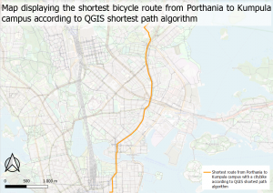
Picture 2.The map showing the shortest route from Porthania to Kumpula using the“shortest path”tool
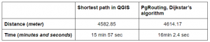
The differences between the analyses are minor which also can be seen in the statistics below in the table. According to the statistics of the analyses, the distance varies slightly as well as the time of travel. The first analysis with Dijkstra’s algorithm has a vaguely longer distance between the start and end vertex than the second analysis. This is probably because of the difference in the start of the route, where the route through Vuorikatu is longer. The time of travel varies by about 5 seconds between the routes so the difference is very insignificant.
Table 2. The table shows the statistical differences between distance and time in the two different network analyses.
A part of the assignment was to create the shortest bicycle route from Pasila train station to Viikki, Kumpula, Porthania, and Aalto campuses. I calculated the time of travel and distances from the station to the campuses with the Dijkstra algorithm. I used the same queries as before (table 1.), besides I changed the start and end vertices for every campus. The Pasila train station is where all the lines meet in the centre of the map and the campuses are at the end of the lines.
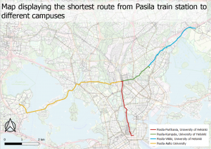
Picture 3. The map shows the shortest path from Pasila train station to the four different campuses calculated with the Dijkstra algorithm
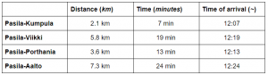
In the table below, I have listed the distances from Pasila train station to the campuses as well as the time of travel. In the assignment, the students arrived at Pasila station at 12 pm so their expected time of arrival is also added to the table. The time of travel was given in minutes but the numbers were in a decimal numerical system. To make it more clear, I converted the decimal numbers into minutes and seconds and then rounded them off to whole minutes.
Table 3. The table shows the differences in route distance and time as well as the time of arrival. The minutes have been rounded to whole minutes for more clarity.
Another task in the assignment was to create hub distances portraying the shortest linear routes from city bike stations to public transport stations. I used the distance to the nearest hub tool to calculate the shortest linear distance. The linear distance doesn’t tell much of the real transport route distance because of the line’s linearity but it gives the relative distances which can be useful when e.g. determining the distance between countries or facilities. The linear distance can also be useful for flight routes and planning infrastructure facilities.
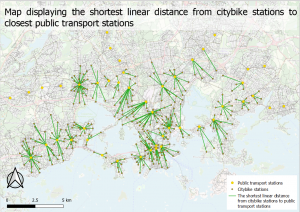
Picture 4. The map shows the hub distance from city bike stations to public transport stations.
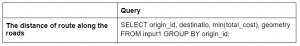
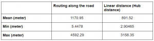
Because the linear distance doesn’t tell much of the transport route distance, the second part of the task was to create the distances of routes along the road. These distances were measurably longer than the linear distances. To be able to perform this analysis, I first made an OD Matrix of all the possible connections between vertices, and then I performed an execute SQL query which calculated the shortest route distances when taking the transport network into consideration. The query I used, is listed in the table below.
Table 4. In the table is listed the query I used to calculate the distances of routes along the road.
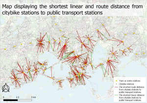
Picture 5. The map shows the shortest linear and route distances from city bike stations to public transport stations
Some city bike stations had a shorter route distance to another public transport station than what the linear distance had suggested. Different obstacles, like infrastructure or construction sites and the environment and so forth, can block the linear distance, thus making the actual route longer. This is fairly normal when it comes to the difference between linear and route distances which needs to be taken into account when calculating distances.
The route distances are useful in navigation and when determining the absolute travel distance with a car, bicycle, or public transport.
I also observed the statistical differences between the two analyses. The values vary a bit, which is expected due to linear distances are often shorter while the route distances are often longer.
Table 5. The table displays the mean, min, and max statistical differences between the linear and route distance.
The last part of the assignment was to create a layer that displayed the city bike stations’ service area with a 500-meter radius and the number of residents within the area. I used the service area tool to create the polygon and afterward, I used the convex hull tool to extract all the YKR centroids within the service area’s polygon. The result of this could be seen in the attribute table, which showed the number of residents inside the service area. Within the service area, there were 457 952 residents.
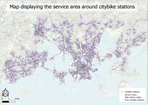
Picture 6. The map shows the service area with a 500-meter radius from the city bike stations.
The results of this extensive analysis were quite realistic. The bicycle routes from Pasila train station to the campuses differed a little bit with Google maps suggested routes and expected travel times. A reason for this may be that Google maps only suggested roads, while my analysis did take walkways into consideration. For example, according to my analysis, the shortest route from Pasila to Kumpula was through Kumpulantaival garden, which is a walkway where motor vehicles aren’t allowed. Google maps don’t suggest this route at all, maybe because the service only suggests roads or roads that have a specific bicycle lane. Data quality is also an important element in network analyses, as incomplete data can severely change and affect the outcome of the network analysis.
Bicycle routes can differ from cars route quite a lot because of the possibility to cycle through places where motor vehicles aren’t allowed. This is important to take into consideration when determining the shortest route and the difference between a motor vehicle and a bicycle route.