
This week’s topic has been raster analysis, focusing on digital elevation modeling and how to do a least-cost path analysis. A least-cost path analysis calculates the shortest, most optimal, and cheapest route from a destination to a source when no network exists. The analysis weights the different inputs and calculates which of those inputs costs more and which of them costs less. This means that some obstacles in the terrain are harder to cross than others, meaning it impacts the cost of the path and thus changes the route. In the analyses, I have used SAGA and GRASS software’s which are integrated with QGIS.
The first part of the assignment was to calculate the slope and aspect degree as well as the curvature of a digital elevation model in the Kilpisjärvi region. This was made with the SAGA terrain analysis geo algorithms. I also calculated the topographic wetness index with the SAGA wetness index (SWI) algorithm. Saga Wetness Index is an index that calculates the soil moisture in a given location. The index is based on the “Soil regionalization by means of terrain analysis and process parameterization” by the EUROPEAN SOIL BUREAU. The SWI algorithm is based on terrain analysis, parameterization, soil regionalization, and then process modeling which is described further in the article. To perform an SWI, a digital elevation model needs to be as elevation input. Also, the type of area and slope must be specified as well as suction. This algorithm results in a topographic wetness index.
The exploratory data analysis shows that there is a positive significant correlation between topographic wetness index and soil moisture. This correlation means that if one of the variables increases or decreases, so does the other variable as well. Therefore, topography affects the soil moisture, for example, if there is a depression in a landscape, there is most likely moist soil in the depression whereas at a hilltop the soil is probably less moist.
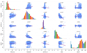
Picture 1. Diagram showing correlations between the variables.
The first least-cost path analysis that I made was with the plugin, least-cost path. It resulted in three paths that don’t take the terrain into consideration. These paths aren’t realistic and therefore I continued the analysis with different methods.
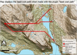
Picture 2. The map shows the least-cost paths when the analysis was made with the plugin
In the second analysis, I used the graphic builder to build a model that took the terrain and different obstacles into consideration when calculating the least cost path. First, I made an analysis where I only used water bodies and slope as inputs, which generated the green route on the map below. Then I ran the model again, this time with water bodies, slope, and also the path network as inputs. This model did also take the path network into consideration when calculating the least cost path which is the dark red route on the map below. Lastly, I made a third analysis where I yet added streams to the model. This resulted in a model that also took streams’ size into consideration, it is the blue route on the map below.
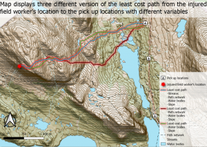
Picture 3. The map shows three different least-cost paths which have different inputs. The inputs used in the calculation of the least-cost paths are listed beneath the symbol.
I calculated the length of all the least cost routes which are listed in the legend on the map. The route which also took the streams into consideration was the shortest route while the route that took the path network into consideration was the longest.
To create a least-cost path analysis, first, a cost surface has to be made. I made the cost surface with the r.series function, which is a raster grid that possesses the cost value of the inputs in each cell. Then a cost distance has to be made, which I made with the r.cost function. Cost distance is a continuous layer with the cumulative cost determining the movement between cells. Lastly, the least-cost path analysis can be made with the r.drain function which I used. Instead of the r.drain function, the r.walk function can also be used to achieve the same results.
This part of the analysis took many hours to complete because the graphic modeler ran for hours before completing the task. At the end of the analysis, the model was quite complex, with many rasterized inputs and functions.
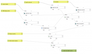
Picture 4. What my model looked like at the end of my analysis.
I did also make a least-cost path with the knight’s move activated in the cost distance section. The knight’s move means that the output will be more accurate but that the process might be slower. Knight’s move doubles the cost distance which means that it covers more grids, meaning that the cost distance with the knight’s move is more comprehensive.
In this least-cost path analysis with the knight’s move activated, I only had water bodies and slope as inputs so the model ran quite fast because of few inputs. The output of this analysis can be compared with the least cost path with the same inputs that I mentioned earlier in picture 3. The map below shows both the least-cost paths with and without the knight’s move and their difference. There is a clear difference between the paths even though they are quite similar. The white path shows a more accurate route, it is 5568 meters long which makes it the shortest route between the injured field worker and the pick-up locations.

Picture 5. The map shows both the least cost path with and without the knight’s move.
Sources:
BÖHNER J., KÖTHE R., CONRAD O., GROSS J., RINGELER A. and SELIGE T. (2002) Soil regionalisation by means of terrain analysis and process parameterisation. Pages, 213-221. EUROPEAN SOIL BUREAU. RESEARCH REPORT NO. 7. https://www.researchgate.net/publication/284700427_Soil_regionalisation_by_means_of_terrain_analysis_and_process_parameterisation
https://helpmanual.io/man1/r.cost-grass/