
My four-month HiLIFE traineeship spanning from furious snowstorms followed by a tender spring awakening to 19 hours of sunshine a day has now come to an end. Not only Helsinki’s residents had to endure extreme temperatures, the plants in my models were also challenged by various climates. In short, I modeled the climate induced species range shift of the flowering plant St. John’s wort (Hypericum perforatum) using a dynamic eco-evolutionary modeling approach. In long, check out my previous Blog Post “Gathering the puzzle pieces for my simulation – The beginning of my HiLIFE traineeship (10th April 2024)”.
And what a journey it has been! I remember precisely how vague the picture of my modeling project seemed during the start of my internship. I crawled through a virtual pile of papers, data, models and ideas. I was wondering how all of that fits together. But every day the picture became more and more clear. And indeed, by the end of my internship I managed to combine all the puzzle pieces and build a shiny simulation. Hurray! At this point: Many thanks to my supervisor Dr Frédéric Guillaume (University of Helsinki) for the support!

But how did I manage to get there?
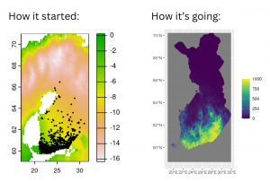
I’m not gonna lie: It was a roller-coaster ride! Shortly after the start I found myself rolling slowly but surely towards the first steep slope: species distribution modeling. Suddenly, scary terms like Random Forest, True Skill Statistic, Pseudo-Absence, and Ensemble Forecast became part of my vocabulary. But it paid off: Fitting a super fancy species distribution model was a true downhill ride (including loopings). Fun! From this distribution model I could derive the occurrence probability of my plants based on the temperature in each location in Finland. Hm, but climate is not the only factor determining species distribution. Land cover also plays a role, or have you ever seen a flower growing on a lake? Me neither. So, I filtered out all the unsuitable locations in Finland.
What’s next? The roller-coaster was already taking off for the next hill to climb: statistically analysing the effect of temperature on characteristics like number of flowers and seed weight. Or in other words, clearing my way through the jungle of Reciprocal Transplant, Resurrection and Greenhouse experiment data (kindly provided by Dr Marko Hyvärinen and Dr Maria Hällfors from LUOMUS, UH, and SYKE). My best weapons were quadratic log gaussian model and negative binomial hurdle model. With those I was able to understand how sensitive my plants are towards temperature. Another puzzle piece!
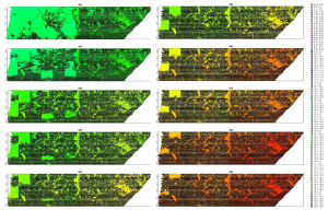
Finally, I was approaching the last bit of this wild roller-coaster ride. Essentially, I was spiraling down towards plugging everything into nemo-age, the simulation modeling tool developed by Dr Guillaume and colleagues. One key aspect here was to include the genetic basics of evolution to allow my plants to adapt to changing temperatures – the heart of a dynamic eco-evolutionary modeling approach. Piecing the puzzle together included a lot of data formatting and tweaking around but I’ll spare you the details. I’d rather join you on a shortcut towards the results of my simulation.
How are the plants doing?
According to my simulations they were doing good and would do even better in the future. That means, the distribution range was predicted to expand north with increasing temperatures. That is quite logical as my data analyses revealed that the St. John’s wort performs better in warmer climates. Additionally, the plants were adapting to the warming climate. This fits well into the general picture that warm adapted plants are predicted to expand northwards (in the northern hemisphere), while cold adapted plants slowly lose their habitat if they are not able to adapt.
So, the simulations confirmed the often-predicted range expansion of warm adapted plants towards the north. The role of adaptive evolution could further be investigated by modifying the evolutionary parameters in the model. But the story of my HiLIFE traineeship ends here. As one might say, all’s well that ends well. The roller-coaster ride as well as the simulations ran through successfully. The flowers in my simulations and in my garden have sprouted. This ride has been a real pleasure and I hope you enjoyed it as much as I did.
– Theresa Koller