
On this page, we will look at the basics of using spreadsheets:
- Feeding data into cells
- Changing row and column sizes
- Inserting and deleting rows and columns
- Hiding rows and columns
Entering data into cells
When you open a spreadsheet program, it will typically create a blank spreadsheet on-screen. You can start entering data into the cells in the spreadsheet rows immediately. You can also import data from other programs (either from a file or the clipboard). When you want to enter data into the cells, go to the cell, enter the data, and accept the cell contents in one of the following ways:
- press Enter, and the cursor will move to the next row down
- press the Tab key, and the cursor will move to the next cell to the right
- press an arrow key, when the cursor will move in the direction of the arrow
- click in another cell with the mouse
- click on the accept button in the formula row (see image below)

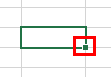
Often, the information you write into a cell is so long that it runs over the right edge of the cell (see example below).

If you are not going to enter any data in the cell to the right, you do not have to do anything about this; you can let the text ‘flow over’ to the next cell.
Automatically filling cells
First, select the cell or cells you want to use as a basis for filling other cells. Then, drag the cell fill handle:
If you want to fill the cells with the same number (for example, 1, 1, 1, etc.), you can do so by typing the number 1 in one cell and then dragging the fill handle down or sideways with the left mouse button.
If you want to fill the cells with a number sequence (for example, 1, 2, 3, etc.), you can do so in the following way:
- Enter the number 1 in one cell. Then press the Ctrl key on the keypad and drag the fill handle down or sideways with the left mouse button.
- Enter the numbers 1 and 2 in two cells. Then drag the fill handle down or sideways with the left mouse button.
If you want to fill the cells with the number sequence 2, 4, 6, etc., you can do so by entering the numbers 2 and 4 in the first two cells. Then drag the fill handle down or sideways with the left mouse button.
You can format a number series after pulling the fill handle and filling the cells. The Auto Fill Options icon appears next to the filled cells.
![]()
Click on the icon to define whether you want to copy the data of the first cell into the cells or to expand the series.
An alternative way to fill cells automatically is to use the Fill button in the Editing group at the Home tab.
Modifying a spreadsheet
If the data you want to enter into a spreadsheet is too long to fit in a column, you have to widen the column. Rows, on the other hand, will expand automatically so that the largest font you are using will fit on a row.
Change column width
When data is entered into the next cell, the end of the text in the previous cell will be covered (see image to the left below). In such cases you have to widen the column so that the whole text is visible (right-hand image).

You can change the column width with Excel by placing the cursor on the right edge of the column header (see image below). The cursor will become a double arrow, and you can stretch the column to its desired width by pressing down the mouse button and pulling the edge to where you want it.

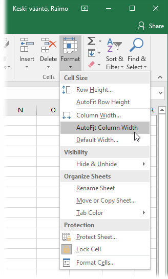
If you want to change the column width to a certain number of points, select the column, then open the Format menu in the Cells group on the Home tab (see image below). If you select Column Width, a menu window will appear where you can set the column width.
If you want the spreadsheet program to automatically set the column width according to the widest cell data, do as described above but select AutoFit Column Width. Alternatively, you you can double-click on the right-hand border of the column identifier. The program will then widen the column according to the widest cell data.
You can change the width of several columns simultaneously by selecting all the columns (by ‘painting’ the column headers with the mouse). Then grab the edge of one of the columns with the mouse and drag it to the desired width. When you release the mouse button, all the selected columns will widen.
Expand rows
The row height will change automatically according to font size, but sometimes you need to change the row height manually.
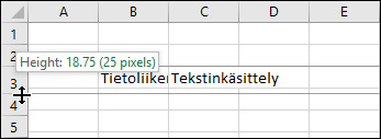
To expand a row in Excel, place the cursor on the lower edge of the row number. the cursor will change into a double arrow. Press down the left mouse button and drag the row to desired height:
When you want to set the row height to a certain number of points, select the row and then open the Format menu in the Cells group on the Home tab (see image under “Expand column width”). By selecting Row Height you can see a menu where you can select the height.
If you want the program to set the row height automatically according to the highest entry, do as described above but select AutoFit Row Height from the menu.
Just like column width, you can change the height of many rows simultaneously by selecting the rows before specifying the height.
Inserting and deleting columns and rows
You can insert new rows or columns anywhere in the spreadsheet. You can also delete rows and columns when necessary.
Inserting a column
With Excel, you can insert a column by clicking on the column header to the left of which you want to insert the column. Then select Insert Sheet Columns from the Cells group on the Home tab.
Deleting columns
You can delete a column by clicking on its column header, and selecting Delete Sheet Columns from the Delete menu in the Cells group on the Home tab.
Inserting rows
With Excel, you can insert a row by clicking on the row number above which you want to add the row, then selecting Insert Sheet Rows from the Insert menu in the Cells group on the Home tab.
Deleting rows
You can delete rows by clicking on the row number, and selecting Delete Sheet Rows from the Delete menu in the Cells group on the Home tab.
You can also insert a column by clicking on a column with the secondary mouse button and selecting Insert from the pop-up menu. To delete a column, click on it with the secondary mouse button and select Deletefrom the pop-up menu.The same principle works for inserting and deleting rows.
Hiding columns and rows
If the number of columns or rows grows very large in a spreadsheet, it may become difficult to find the information you want. In such cases, it makes sense to hide the columns and rows that you are not immediately interested in.
With Excel, you can hide a row or column by selecting the row(s) or column(s) and then opening the Format menu in the Cells group on the Home tab (see image below). Select either Hide Rows or Hide Columns from the Hide & Unhide menu.
To bring back a hidden row or column, select the row numbers or column headers on either side of the hidden row/column, then select Unhide Rows or Unhide Columns from the Hide & Unhide menu in the Format menu.
Sorting
Sometimes part of a spreadsheet may need to be sorted in rows in ascending or descending order. In this case, first select the area to be sorted from the table, and then select the Sort action from the Data tab. Next, under Column – Sort by, select the column containing the values on the basis of which the rows of the range are sorted and under Order, select the ascending or descending order. If necessary, you can sort the rows by values in more than one column (for example, firstly, by people’s last names and secondly, by their first names).