
EXERCISE 1 – Good routines for spreadsheet calculation
- Reread the page on good routines for spreadsheet calculation.
EXERCISE 2 – Creating and modifying a spreadsheet
| In this exercise, we will create a spreadsheet for a student budget. |
- Create a new spreadsheet by opening File and selecting New.
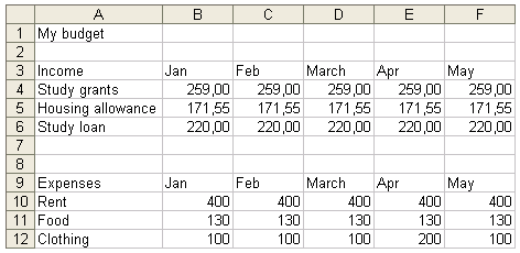
- Create a spreadsheet according to the model below. Enter your true income and expense data in your spreadsheet (substitute e.g. “Clothes” with other expenses you have).
(A verbal description: in the cell A1, it reads “My budget”. In the cells A3 – F3 we have “Income”, “Jan”, “Feb”, “March”, “Apr”, “May”. In the cell A4, it reads “Study grants”, in A5, “Housing allowance”, and in A6, “Study loan”. In rows 4 – 6 and in columns B – F, there are some sums in euros. In row 4, all these sums are 259.00; in row 5, 171.55, and in row 6, 220.00.
In the cells A9 – F9 we have “Expenses”, “Jan”, “Feb”, “March”, “Apr”, “May”. In the cell A10, it reads “Rent”, in A11, “Food”, and in A12, “Clothing”. In rows 10 – 12 and in columns B – F, there are some sums in euros. In row 10, all these sums are 400; in row 11, 130, and in row 12, 100.) - Save the spreadsheet in your home directory under the name My budget.
- Modify the spreadsheet regularly, keeping track of your income and expenses. If you are receiving the student grant from KELA, you can check how much you are allowed to earn on their web site!
EXERCISE 3 – Cell settings
| In this exercise, we will modify the spreadsheet we created in the previous exercise. |
- Open the workbook My budget that you created in the previous exercise, unless it is already open.
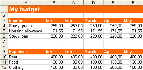
- Modify the spreadsheet according to the model below (choose the colours you want).
- Set the spreadsheet to show two decimals.
- Save the changes you made to the workbook.
EXERCISE 4 – Creating the most common formulas
| In this exercise, we will practise using different formulas. |
- Open the workbook My budget unless it is already open.
- Add up the income from January; enter the word Total in cell A7 and create the formula for the sum in cell B7 with the help of the AutoSum button in the toolbar.
- Copy the formula to the other cells on row 7.
- Sum the January expenses; enter the word “Total” in cell A13 and use the AutoSum button again to create the formula in cell B13. Copy the formula to the other cells on row 13.
- Calculate the sum remaining after expenses in January: enter “Savings” in cell A15 and create the formula to calculate the savings in cell B15. Copy the formula to the other months.
- Calculate the row sums in column G: enter “Total” in cells G3 and G9 and create the formula for the row sum in cell G4. Copy the formula to the other cells in column G.
- Add the borders as in the model to the “Savings” row.
- Save the workbook.

EXERCISE 5 – Cell references
| In this exercise, we will use both absolute and relational cell references. |
You suddenly realise that you have other expenses that you want to add to your budget. You are also planning a trip in the summer, after the term ends. For this end, you have to work to earn the money for the trip. You want to use this spreadsheet to calculate how many hours you need to work each month in order to earn enough. Your employer has offered you 12 euros/hour (in this exercise, we do not take taxes into account). The trip will cost a total of 800 euros.
- Open the workbook My budget.
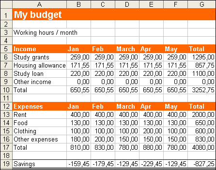
- insert a new row above row 13. Enter the following data on the row:

- Add two new rows above row 3 and enter the data below on them:
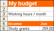
- Add another row above row 9, and write the title “Other income” in cell A9 (see next image). Create a formula for row 9 to calculate how many hours you need to work to make the money last.
- Create a formula in cell B9 to calculate working hours x 12. Make the cell address of B3 absolute so that you can copy it to the other months. Copy the formula to the other months.
- Copy the Total formula in G8 to cell G9 beneath it.
- You added a new row above the “total income” row, but the program did not update the cell addresses automatically, so you have to correct it. Place the cursor in B10 and correct the address for the calculation range on the formula row. Copy the corrected formula to the other months.
- Now you can enter in cell B3 the number of working hours you thought might be enough to save 800 euros for the trip.
| In this exercise, we will practise using absolute references when the dividend changes but the denominator remains constant. Save the “Number of students”-file in your Spreadsheets folder (if you have not created this folder before, create it in your home directory now). |
The spreadsheet shows the number of new students and all students at different universities in a certain year. You want to calculate how many ‘old’ students there are in each university.
- Open the exercise ‘Number of students’ and add a new column to the left of the column ‘Old students’.
- Enter the heading ‘Old students’ in cell B1 (you can divide the text onto two rows by pressing Alt+Enter between the words).
- Create a formula in B2 for subtracting the value of the cell ‘New students’ from the value of the cell ‘Old students’ (use cell references in your formula).
- Copy the formula to the rows beneath it.
- Enter the heading ‘Total* in cell A22 and calculate the number of old students. Copy the formula to the other columns.
- Next calculate how many per cent of the total number of students the students of each university make up: enter ‘Percentage’ in cell E1 and create a formula in cell E2 to calculate how many per cent of the total number of students the students at UH make up (=Uh students total / all students total). Change the address of the ‘All students total’ cell to an absolute address so that it does not change when copied.
- Copy the formula you created to the other rows.
- You will see the correct answer in the Solution spreadsheet in the workbook.
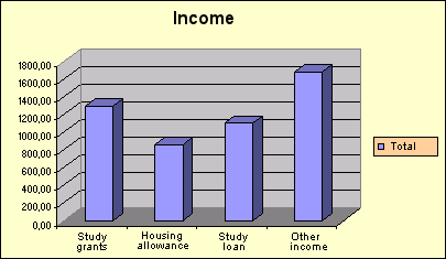
EXERCISE 6 – Creating graphs
| In this exercise, you will try to create graphs. |
- Open the workbook My budget again.
- Create a graph like the model below on the basis of the budgeted income in the spreadsheet. Place it after the spreadsheet.
- Create a graph of the expenses according to the model below and place that, too, in the spreadsheet after the data.
(A verbal description: the graph is a 3-D pie chart with the title “Expenses”. There are sectors for rent, food, clothing, and other expenses. Next to each sector it says what this sector is about, and what is its share of the total expenses (e.g. “Rent 49%”). In addition, there is a legend at the bottom displaying the meanings of the sector colors.)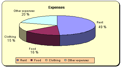
- Analyze your graphs critically:
a) Is the student grant over or under 1,200 in the bar chart?
b) how do you think the pie chart displays food expenses? - Save the changes to the workbook.
ANSWERS
EXERCISE 6 – Creating graphs
In exercise 4, it is hard to estimate how much the student grant is because the graph is three-dimensional, and the percentage of food expenses looks much larger than the expenses for clothes in the pie chart, though the percentages written beside the chart show that there is not much difference. If you use this kind of graph, you will have to enter the numbers, as well. These graphs show that it is hard to interpret three-dimensional graphs.