
The basic idea of a spreadsheet program is that it allows you to do different calculations using the cells in the grid. As all calculations are performed using formulas, you can change the numbers in the calculations at any time and let the program redo the maths for you.
A formula begins with an equal sign (=). After the sign, the formula contains the cell addresses and maths operators included in the calculations.
Cell address
In a spreadsheet program, each column and row has its own identifier. These identifiers together form the address of a cell:
- Columns are identified by letter in alphabetical order: the first column is “A”, the second is “B”, etc. After Z, the column identifiers continue as AA, AB, AC, etc.
- Rows are identified by a number: the first row is “1”, the second is “2”.
- The cell address is formed from the column indicator and the row identifier: for instance, the address of a cell in the second column on the first row would be B1.
Making a formula
In its simplest form, making a formula only requires that you enter the maths operator and the addresses of the cells used in the calculation.
Always use cell addresses in formulas instead of the number entered in the cell! This allows you to easily copy formulas and change the numbers in the cells referred to in the formulas.
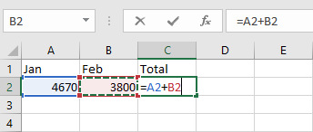
In the example below, cells A2 and B2 are added together. The steps to creating a formula:
- Move the cursor to the cell in which you want to see the result of the calculation
- Start the formula with the equal sign =
- Click the cell A2 with your mouse (follow the formation of the formula on the fx row as seen in the picture)
- Use your keyboard to enter the + sign
- Click the cell B2.
- Accept the formula by pressing Enter or click the OK sign on the fx row:

P.3 – Making a formula in Excel – text equivalent
You can edit functions and formulas in the formula bar above the columns.
Common maths operators
The maths operators most commonly used in spreadsheet calculations include:
- + addition, example formula =A1+B7
- – subtraction, example formula =A5-A8
- * multiplication, example formula =B6*B8
- / division, example formula =A5/A8
The calculations are performed according to normal operator precedence: multiplication and division are performed first, followed by addition and subtraction. However, parentheses can be used to change the order of operations. The program will perform any calculation in parentheses first. For example, in the formula =A4*(B3-B5), the first calculation is the subtraction inside the parentheses.
The calculations in formulas is always performed using the exact value of the number contained by a cell. Thus, even if you specify a number in a cell to be shown with two decimal places (showing the number 0.34444 as 0.34, for instance), the exact value 0.34444 will always be used in the calculations.
Common functions
In addition to the most common operators such as addition, subtraction, multiplication and division, spreadsheet programs contain a great number of different functions. Functions are predefined formulas.
The most commonly used function is the Sum function used to calculate the sum of the values within the range of the formula. You can use the Sum function instead of the operator +, making it easier to write down the formula.
The most common functions are conveniently placed under one menu in the Formulas tab. Click the small triangle under the Autosum icon to open the menu shown in the image below. Along with addition, the menu contains a function to calculate the Average of a series of numbers.
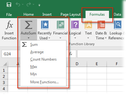
Selecting “More Functions” opens a box where you can search for functions either by keyword or by browsing them by function category. For example, there are statistical, mathematical, trigonometric, financial, and date and time functions available. If you select the function to be used in the formula this way, Excel can help you use it. Alternatively, you can write the name of the function in your formula. Note that if the Excel language is set to Finnish, the functions must also use their Finnish names! For example, the function Sum is Summa in Finnish. A few examples of other frequently needed functions: Average, Median, Min, Max, Correl.
Functions perform their tasks according to the arguments given to them. The arguments are written after the name of the function inside parentheses. Their number depends on the function used, but many common functions have only one argument. It is often used to assign the cells whose values it must use in its operations to the function. A range of cells can be defined by indicating from which cell address it begins and where it ends. A colon is written between these addresses. For example, the sum of the values in cells A1, A2, A3, and A4 would be given by =Sum(A1:A4) or, if the language of Excel is Finnish, =Summa(A1:A4). The range given as an argument can also be inconsistent if a semicolon is used to define it: e.g. =Sum(A1:A4;C7) or =Sum(A1:A4;C7:F7).
In Excel, the Sum function is available as a button in the toolbar. With this Sum function you can add the
values of an area in the spreadsheet as follows, for example:
- Place the cursor in the cell where you want the result of the sum.
- Click on the AutoSum button.
- The program will suggest which area to sum: if it is correct, you can accept the formula by pressing Enter; if it is not, select the area with the mouse and then accept it with Enter (see image below).
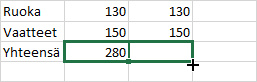
- If you so wish, you can use the Fill handle to copy the formula to other cells.
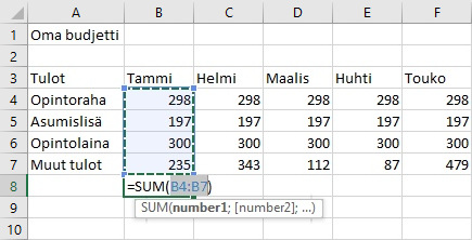
Always check the area that the program suggests; the program will only select an uninterrupted area automatically, so if there are empty cells in the area, it will not select the cells on the other side of them!
You can also do sums as follows: select the cell area you want to add, and include the empty row or column where you want the result to be shown. Click on AutoSum. This feature only works to the right and downwards.
Copying formulas
You can copy a formula you have created to other cells. If, for example, you have calculated your student allowance for each month separately, you only have to create a formula for the January row. Then you can copy the formula to the other months.
With Excel, formulas are copied with the so-called Fill handle; the Fill handle is located in the bottom right corner of an active (selected) cell. The stages of copying a formula:
- Activate the cell from which you want to copy the formula.
- Place the cursor on top of the Fill handle. You will see that the cursor changes into a black cross.
- Press down the primary mouse button.
- Pull the Fill handle in the direction in which you want to export the formula.
- Release the mouse button in the last cell where you want to copy the formula.
Take a look at the video below to see how to easily create and copy a sum formula in Excel!